
Valuation Adjustments - XVAs

Valuation Adjustments, XVAs for Derivatives
Valuation Adjustments (VAs) have been part of financial markets for many years.
More recently, the calculation methodologies for VAs have been significantly advanced and are now very quantitative involving complex models across a wide range of VAs.
As the number of VAs has expanded, they are collectively described as ‘XVAs’.
This blog is the first of a series which explains the types, uses and calculation methodologies for many XVAs. The blogs will not cover all the XVAs but will describe those frequently encountered by clients. The calculation methodologies are described in basic terms without excessive detail: if you want that level of explanation, feel free to contact me. The calculations in most XVAs vary from analytic approximations to full simulations.
This blog introduces some XVAs I regularly see for clients.
Following blogs will look at each XVA in more detail covering uses and calculation.
Why are XVAs important for derivatives?
Derivatives (e.g., interest rate swaps) have characteristics which are different to other assets and liabilities:
They have 2-way exposures, you can have payments or receipts
ii.This makes the calculation of exposure sensitive to market levels and future directions
The calculations and approaches are therefore different and often more complex than one-sided exposures such as bonds.

Bond - Cashflow is fully at rsk at default at any price

Derivative - Cashflow is not fully at risk at default because it is offset by an opposing cashflow dependent on price
Note: Some XVAs are applied to collateralised transaction and some to uncollateralised transactions.
CVA – Credit Valuation Adjustment
CVA = -LGD * ∑ (EPE * PDc)
LGD = Loss given default (assumed to be 40%)
EPE = Expected discounted positive exposure where only positive exposures are included
PDc = Probability of default of counterparty (market input)
Calculation is done in discreet time steps so that the EPE and PD are specific to that time step, and this is summed over the entire trade until maturity.
Applied to uncollateralised transactions.
DVA – Debit Valuation Adjustment
DVA = -LGD * ∑ (ENE * PDs)
LGD = Loss given default (assumed to be 40%)
ENE = Expected discounted negative exposure where only negative exposures are included
PDs = Probability of your default (market input)
Only used for accounting and generally for corporates.
Applied to uncollateralised transactions.
FVA – Funding Valuation Adjustment
FVA = ∑ (EE * FSs)
EE = Expected exposure, sum of EPE and ENE
FSs = Your funding spread
Calculation is done in discreet time steps so that the EE and FS are specific to that time step, and this is summed over the entire trade until maturity.
No LGD used
Applied to uncollateralised and some collateralised transactions.
KVA – Capital (K) Valuation Adjustment
KVA = ∑ (EC * CC * ti)
EC = Discounted expected capital profile
CC = Cost of capital
This is often a theoretical calculatio. Most banks replace KVA with RoC (Return on Capital)
MVA – Margin Valuation Adjustment
MVA = ∑ (EIM * FSs * ti)
EIM = Discounted expected initial margin (often calculated from ISDA SIMM)
FSs = Your funding spread (as per FVA)
Used only for collateralised transactions
CollVA – Collateral Valuation Adjustment
ColVA = ∑ (ECB * FSs * ti)
ECB = Discounted expected collateral balance (EE from FVA)
FSs = Funding spread of collateral x relative to discount rate
Applied to collateralised transactions.
Discount rate is the actual rate in your system, e.g., SOFR
FSs accounts for different collateral and currency
Is usually very idiosyncratic – it is your cost of collateral
E.g., discount cross currency against SOFR (mkt standard) but collateral is in JPY
Summary of Valuation Adjustments, XVAs
Uncollateralised
CVA (always a cost)
DVA (always a benefit)
FVA (cost or benefit)
Collateralised
MVA (always a cost)
CollVA (cost or benefit)
FVA (if term funding is required)
Both
KVA (always a cost)
Trade execution methodologies and strategies
This is the first in a series of blogs which will look more closely into some successful approaches to designing effective derivative and FX trade execution strategies for clients. “Effective’, in my definition is a fair outcome for both sides of the transaction which also minimises any chance of offending regulatory and legal requirements.
For example, pre-hedging is one strategy that I have found very useful (when managed correctly) to reduce risks and achieve positive outcomes for clients. It is particularly effective in managing large trades and/or illiquid markets to avoid adverse price movements.
We have written previously on the topic of ‘pre-hedging’ and how this challenging matter can present both buy and sell-side market participants with real decisions.
This blog looks at identifying a preferred outcome, developing a series of potential strategies and deciding on the appropriate strategy to follow. Future blogs will look at examples of alternative strategies, how to you may choose to implement these strategies and managing counterparties.
Identifying the preferred outcome(s)
The first step is to identify and internally agree the preferred outcomes. Basically, if you do not know and agree how you want this to end, it is hard to make plans that support that end.
Some outcomes could include:
Is there a specific price or level that is important to hit?
In some cases, there is a price point that delivers an outcome which is required for cashflow, target price, accounting simplicity etc.
Do you have any counterparties you have to include?
Sometimes relationships and/or other dependencies on a counterparty may mean they need to be part of any trade.
Are there any other counterparties you would like to include?
Is there a balance between best price and relationship?
Are there any internal parties that need to be included in decisions?
For large transactions, the board may need to be informed, and they may have some specific requirements.
Prioritise the preferred outcome(s)
The next step is to prioritise the preferred outcomes.
If you have more than one preferred outcome, then they will need to be prioritised.
In most cases, you will need to compromise on lower priority outcomes if you need to meet the highest priorities.
Look at alternative strategies to achieve the preferred outcomes
There are many ways to achieve the outcomes, but a strategy suited to the market liquidity conditions, counterparties and preferences will greatly improve the probability of a favorable outcome.
Some of the strategies include:
Single counterparty only for the trade
Running a tender involving several potential counterparties
Using a syndicate of banks who all get some of the trade
Using a single bank to execute the hedge before novating the hedges to a syndicate of banks
Single bank to arrange a pre-hedge the trade before novating to a syndicate of banks
Etc.
And note, each strategy has merits and challenges!
Deciding which strategy to adopt for this transaction
It is important to match the strategy to the preferred outcome.
Not all strategies will be effective for all outcomes
So, a decision will need to be made as to the best strategy in this situation.
Summary
The better approaches spend time and effort on making sure the outcomes are well understood (and agreed) before proceeding to the strategy to get the best chance of achieved that outcome.
Not all situations are the same so matching the strategy to the conditions is also important.
The next blog will look at examples of the strategies above. I will look more closely at the merits and better uses of each strategy and the ways they may be used to get an effective outcome.

Pre-hedging and the use of electronic execution platforms

Recently we published a podcast on the Martialis website where I discussed the development and use of electronic execution platforms with Anthony Robson. Anthony was CEO of Yieldbroker where they created the electronic trading infrastructure over 20 years and serviced the fixed income markets in Australia.
One of the topics we explored was the role of electronic execution platforms for pre-hedging of client trades by market participants. This has been a very important subject recently.
FMSB published ‘Pre-hedging: case studies’ in July 2024 which looked at the role of execution platforms in pre-hedging.
This blog looks at the FMSB case studies and relates the relevant example to my conversation with Anthony.
Recap on recent guidance on pre-hedging
Several industry and regulatory groups globally have provided guidance on pre-hedging in financial markets. We have reviewed them in previous blogs which can be found here, here, here, and also here. As you can tell, we have been busy in this subject!
One of the earliest examples of global guidance was within the FX Global Code first published in 2017. Principle 11 specifically addressed pre-hedging and was updated in 2021.
The FMSB has also updated their guidance in 2021. This has been recently supported by some case studies which are designed to assist market participants identify and manage pre-hedging activities.
The Australian regulator, ASIC, has also weighed in with a ‘Dear CEO’ letter published in February 2024. ASIC proposed 8 points which sell-side firms may use in any pre-hedging activity.
However, any advice or guidance can only assist market participants and will be subject to local regulatory and legal requirements. In other words, all market participants should pay close attention to the specific situation and their involvement in pre-hedging.
Most guidance emphasises any pre-hedging should be designed to:
Benefit the client or, at least, not adversely impact that client.
Be done with reasonable expectation of winning the trade. Note that a trader knowing they will win the trade in the very near future may not be consistent with ‘reasonable expectation’ and may constitute front running.
The role of electronic execution platforms
Returning to the FMSB, the 2024 case studies include 4 different examples of pre-hedging.
Case studies 1a, 1b and 1d all include using an electronic platform as the execution method. In all cases the client order is sent as a ‘RFQ’ (Request for Quote) in a liquid or illiquid market or product. The banks receiving the RFQ react in different ways based on whether it is a 1 or 2-way price request and/or by either pre-hedging or not. The trade is awarded to a single bank in each case.
The challenges for the banks receiving the RFQs on electronic platforms include:
Potential for the information to leak from the pricing desk to other traders thereby providing them with non-public information.
Pre-hedging may be permissible as long as it follows points 1 and 2 in the previous section.
While the time to respond to a RFQ may be very short (seconds typically) manual pre-hedging is impractical but algorithmic trading can quickly access electronic platforms. This needs to be carefully considered by banks and clients.
Illiquid markets and products present special challenges. While attempting to manage the possible position from winning the RFQ, a bank may impact the market price substantially.
I also note that the FMSB case studies include some client responsibilities to communicate clearly and honestly and be very clear about whether they accept any pre-hedging activity.
It is important to note that obligations and responsibilities impact both the intermediary (bank) and the clients.
The benefits of electronic platforms
The podcast with Anthony really highlighted using electronic platforms can have major benefits in managing risks as well as compliance with market obligations.
In the example of Yieldbroker (and I assume most platforms I have used), the electronic records of all activity are collected as a matter of routine.
There is a complete audit trail of activity that can be used for checks and analysis.
Platforms are generally required to conduct some form of surveillance to identify unusual behaviors or potential market abuse.
Orders and RFQs can be explicit about whether pre-hedging is permitted and record that agreement.
While it is possible to use another platform for pre-hedging apart from the one with the RFQ, it is possible to collect data from many platforms, check the time and activity and cross reference the pricing and trading.
Is pre-hedging permitted?
The simple answer is yes, provided it follows the rules and is agreed to by both parties.
Electronic trade execution platforms are often the dominant form of RFQ and trade execution especially in FX and fixed income markets. As such they have an important role and have functionality and characteristics which differ from voice markets.
How much is traded on electronic platforms?
The market data on turnover is difficult to gather accurately because it is spread across a number of different reporting entities including CFTC, ESMA, BIS, industry bodies such as ISDA as well as the platform providers.
However, it is generally understood that:
US and European markets trade approximately 70 – 90% of interest rate derivatives electronically due to regulatory requirements.
Around 30 – 50% of non-spot FX is traded electronically.
75 – 85% of spot FX is traded electronically.
I do note that these percentages can vary widely across regions and currencies but represent a significant proportion of the traded risk.
With relatively high percentages traded on electronic platforms, perhaps the FMSB focus on pre-hedging cases on those platforms is timely and relevant.
Summary
Electronic platforms for executing derivative and FX trades are well established and commonly used by market participants.
FMSB has recognised this and has recently provided a number of case studies of pre-hedging which related directly to the use of such platforms.
My discussion with Anthony Robson was very useful in understanding how the platforms are used and how they can provide great data for analysis of trading patterns. The complete audit trail including orders and trades can help identify when participants are trading and in what manner.
Electronic platforms are commonly used for trade execution and are very amenable to algorithmic trading: this aspect can create additional risks for market participants and may require additional controls.
In the case of pre-hedging, this could be detected by platform analytics and particular care needs to be exercised by all market participants to align their obligations to clients and markets with their trading patterns.
All the guidance in the world…
In February, ASIC released their Dear CEO Guidance for market intermediaries on pre-hedging setting out the Commission’s expectations in relation to a market practice that’s increasingly in the spotlight.
This was making good on a promise of ASIC Chair Joseph Longo, who back in 2023 noted industry’s “calls for guidance” on this thorniest of topics.
In this blog I ask a simple question: when it comes to pre-hedging, does ASIC’s (or anyone else’s) guidance matter?
‘Principles and guidance are great but they’re not enforceable. ‘
With these word’s the US-based Managing Director of a major global market association neatly summed up the rather uniquely Australian pre-hedging conundrum. Faithfully abiding by industry and regulatory guidance might be helpful, but it is only partially helpful if your trading patterns and deal outcomes appear to put you on the wrong side of the Corporations Act.
And what happens if you are on the wrong side of the Corporations Act, inadvertently or otherwise?
What we know is that it is the Corporations Act that matters. While pre-hedging situations may be rare, any ASIC investigative and/or enforcement action carries risk and almost certain business disruption (that can carry for many years).

ASIC’s Guidance
We‘ve blogged on this topic a lot in the past year, with John Feeney’s February post arguably the best of available summaries and one that helpfully provides a kind of guidance on the guidance.
Here I plagiarise in order to recap John’s points of what constitutes best practice in ASIC’s view:
Document and implement pre-hedging policies and procedures to ensure compliance with the law.
Provide effective disclosure to clients of the intermediary’s execution and pre-hedging practices in a clear and transparent manner – before any pre-hedging is conducted.
Obtain explicit and informed client consent prior to each transaction.
Monitor trade execution and client outcomes and seek to minimise market impact from pre-hedging.
Appropriately restrict access to and prohibit misuse of confidential client information and adequately manage conflicts of interest.
Have robust risk and compliance controls, including trade and communications monitoring and surveillance arrangements, to provide effective governance and supervisory oversight of pre-hedging activity.
Record key details of pre-hedging undertaken for each transaction (including the process taken).
Undertake post-trade review to determine the quality of execution for complex and/or large transactions.
ASIC went on to reminded CEO’s that:
‘failure to live up to these standards can be unfair and unconscionable.’
The market response?
It’s fair to say that the Dear CEO letter generated a lot of market interest and discussion among domestic and international firms alike. Some feel that ASIC has inserted a new higher standard with point seven.
For others, the insertion of point seven signalled the creation of what amounts to a uniquely Australian arrangement.
To recap ASIC’s pre-hedging guidance, point seven:
7. Record key details of pre-hedging undertaken for each transaction (including the process taken).
This is a definite extension of the guidance provided by both the FMSB and within the FX Global Code.
FMSB - Standard for the execution of Large Trades in FICC markets
Global Foreign Exchange Committee - Commentary on Principle 11 and the role of pre‐hedging in today’s FX landscape
And it doesn’t matter how large the underlying transactions are, the Corporations Act is in force down to the cent. The key point here is that the legislation does not appear to only refer to ‘large transactions’.
What are some of the practical risks and difficulties this creates?
It’s important to remember that when dealers are engaging in pre-hedging, they’re doing so as principals – i.e., as principal risk takers. They are also operating in risk-transfer settings, typically with multiple stakeholder interests to consider as they go about serving customers, managing an order book, and their firm’s own risks.
We also note that the dealing environment can vary between quiet periods of relative inactivity and periods of high turnover and volatility. In the latter the exercise of dealer discretion and split-second decision making are very normal, for example when market data is released or there is significant news flow.
We ask:
How do firms treat trades conducted in proximate time and price around the level of those that are recorded as pre-hedges for a specific transaction?
Is there a risk that by specifying a who-gets-what requirement for individual fills that a situation evolves where there is (real or perceived) ‘good-trades for us bad-trades for the client’ event ?
Which makes us think pre-hedge transactions should probably be recorded contemporaneously with a compliance operative present? But gosh, that adds a whole new layer of dealing oversight, complexity, and potential disruption.
We also ask, what if after all of the best compliance with ASIC guidelines, the market moves adversely against the client’s interests regardless?
There appears to be no easy answer to these questions.
So, does ASIC’s (or anyone else’s) guidance matter?
We’ve mentioned previously that we believe market intermediaries now bear a disproportionate responsibility for conflict-free, non-disruptive risk transfers in financial markets.
The latest ASIC guidance appears to add further to that burden.
We are also on the record as encouraging the development of guidelines for those who bring deals on the buy-side. But such guidance seems unlikely to emerge, at least any time soon.
In the absence of some new move to amend the Corporations Act, we therefore encourage firms to follow the guidelines with clarity, and think particularly carefully about:
documenting pre-hedging policies and procedures
recording the details of pre-hedging undertaken for each transaction
Our own mantra is worth remembering:
‘If it’s not written down it doesn’t exist.’
If it doesn’t exist, you probably have a risk you don’t need.
So yes, the guidance matters, and it matters a lot since a failure to demonstrate compliance will surely count against firms that become exposed to post-deal investigations.
The ability to demonstrably show compliance with the ASIC guidance may be all that actually protects a firm
Pre hedging and trading: A practical guide and recent experiences of balancing outcomes
With the recent regulatory interest in pre-hedging, there has been a predictable focus on how this will impact both sides of the market: buy and sell. The ASIC letter to CEOs and the impending IOSCO guidance will add to the existing FMSB and Global FX Code publications.
At Martialis, we have recently worked with intermediaries (i.e., banks) and their clients (corporates and non-bank financials) to look at the practical ways to manage trade execution within the regulatory and market practice guidelines.
This article summarises our recent experiences where the balance between the banks and their clients is managed for derivative transactions.

The buy-side
Buy-side clients are always very much on top of their balance sheet exposures. They really understand the funding and liquidity needs for their businesses and frequently use derivatives and FX to hedge exposures.
They often use derivatives as hedges against liabilities. The derivatives of choice are interest rate and/or cross-currency swaps which can be relatively simple or complex. The swaps can be restructures of existing positions or traded as new swaps.
In restructures, the same counterparty as the original trade must be in the conversation. Our observations have shown repeatedly that some banks do add cost to the trade simply because the client has little choice of counterparty; that is, they are ‘captured’.
New trades are different, they can be shown to a variety of banks and the competitive tension is much more clearly reflected in new deal pricing. The prices tend to be more aggressive, perhaps reflecting the approach that getting the deal allows for restructuring later (see the previous paragraph).
The sell-side
Banks and intermediaries have a tough balance to maintain: what is a realistic price, and does it cover my costs and required returns?
This balance can be difficult to manage and can lead to the typical dilemma: How do banks get to an attractive price while meeting target returns?
How does a trader manage risks in an existing book while not creating an inappropriate market impact that may be (or perceived to be) pre-hedging?
Sales staff are equally challenged to maintain the relationship with their client while only divulging the minimum, appropriate information to traders. Clearly there needs to be some communication, but what is considered ‘appropriate’?
In many cases, the sell-side is considering carefully the management of all trades with clients to balance the regulatory requirements.
What are we seeing?
Pre-trade market moves certainly appear to be happening, and we have seen such price moves in markets just prior to trading.
The price moves may not be associated with any potential counterparties, but it happens often enough that may not be a coincidence.
Is it pre-hedging? We cannot be certain.
Strategy is everything. For the buy-side, agreeing a clear approach before talking to any bank is imperative. As soon as we ‘break cover’ there is a possibility markets move against the client interest and/or we place banks in a position which amplifies the potential conflicts of interest.
Limiting the information provided to the banks and the timing of the release of that information can reduce risks (and costs) for both sides of the trade.
Dry runs are a must. The dry run will help align the pricing especially for restructures and complex trades. This gives us time with the client to identify outliers and negotiate the pricing well before the trade execution time.
Keep the actual execution time confidential for as long as possible. Dry runs help get pricing issues resolved but keeping the actual date and time of trading confidential minimises the potential for market moves related to the trade.
XVAs (CVA, FVA and possibly KVA) need to be priced independently. Banks can layer additional spreads into KVAs. This may be done by individual bank staff or as a corporate policy.
Getting an independent price for the trades and the XVAs before talking to potential counterparties gives our clients the ability to identify any anomalies and confirm the actual spreads they will be paying.
Just comparing prices from different counterparties is not very effective because differences in details which impact prices can go undetected. Getting a full breakdown of the trade mid and spreads means both sides can confirm the details and minimise the chance of miscommunication.
SummarY
Moves in markets just prior to trades for buy-side clients do happen. And it occurs with sufficient regularity to suggest this is not entirely coincidence. Whether this is pre-hedging or not is an open question.
However, if a bank is involved in a trade where the markets moved just prior to the execution of the trade, we recommend they look at whether there was any involvement by their traders. The activity may be unrelated, but it is better to confirm this at the time via an independent review.
A very effective sell-side practice is to look at the trade from the perspective of the client. If they intentionally move a market or pre-hedge, this may be ok if the client benefits overall. But be clear about this before the trade and review after the trade.
We are yet to see any disclosure from banks that they may pre-hedge a trade. At best it appears in the disclaimers (in the small print) but has not been explicitly discussed in our experience.
We continue to work with many market participants on both buy and sell side firms. Our best advice is to get independent and informed advice on the strategy and pricing before executing trades.
Some practical approaches to ASIC’s February 2024 letter on pre-hedging - Part 2
We published a blog in February 2024 which looked at the content of the ASIC letter for market intermediaries on ‘pre-hedging’.
That blog was focused on our interpretation of the ‘Dear CEO’ letter which was written to many banks and intermediaries. In most cases, as is normal for ASIC, the firms were required to provide a response.
A significant challenge for intermediaries is the practical application of the contents of the letter. This is further complicated by firm’s obligations under the FX Global Code and the FMSB guidance on handling large trades which offer similar but subtly different guidance to that in the ASIC letter.
It should be noted that many market participants have signed up to the FX Global Code and/or are members of the FMSB so are bound by those publications.
In addition, IOSCO is due to publish the results of a survey on pre-hedging later in 2024. This will likely add to the mix of guidance and will have the backing of many global regulators (including ASIC) who are IOSCO members.
All the codes and guidance have overlaps but also have some differences. This is to be expected because each jurisdiction is bound by their legislation and regulations which can and do differ across regions.
So, what is an intermediary to do? This blog looks specifically at the ASIC guidance and offers some practical alternatives for firms to consider when looking to comply with the Australian requirements.

Our summary of the ‘Dear CEO” letter from the previous blog
We provided this summary in the previous blog. It is a useful starting point for practical ways to address the point in the letter.
‘While consistent with global equivalents, the 8 points provide intermediaries with clear reference to the relevant Australian legislation and regulatory guidance.
It is very important to note that this is Australian guidance, and it may not be identical with other jurisdictions due to the local environment.
The challenge for many firms is the practical implementation of the contents of the letter.
How do you define which transactions will require explicit client consent to pre-hedge?
Who is an informed client and who may need additional assistance to fully appreciate the implications of pre-hedging?
How do you define and measure market impact when markets can vary in both the liquidity and the participants in each product?
How do managers oversee the pre-hedging and ensure it is consistent with regulation and guidance?
Since the guidance is a ‘Dear CEO’ letter, how does a CEO ensure compliance?’
The summary poses 5 questions which we believe are important for intermediaries to consider for pre-hedging.
We now look at each question related to the 8 points provided by ASIC and offer some practical ways to address the contents of the letter.
The 8 ASIC points with thoughts on a practical approach to compliance
The 8 separate points follow which make up the guidance. The ASIC extracts are in italics and our views are in normal script.
‘document and implement policies and procedures on pre-hedging to ensure compliance with the law. They should ideally be informed by consideration of the circumstances when pre-hedging may help to achieve the best overall outcome for clients.’
Update the current policies and procedures with reference to pre-hedging if there is no explicit mention.
This could be assisted by using pre-hedging in the examples.
Provide updated training to impacted staff which specifically includes pre-hedging as a worked example.
2. ‘provide effective disclosure to clients of the intermediary’s execution and pre-hedging practices in a clear and transparent manner. Better practice includes:
·upfront disclosure, such as listing out the types of transactions where the intermediary may seek to pre-hedge; and
post-trade disclosure, such as reporting to the client how the pre-hedging was executed and how it benefitted (or otherwise impacted) the client;’
Include an explanation of the pre-hedging practices (that this may occur) in the pre-trade discussion and written material.
Include the specific instruments that may be accessed for pre-hedging.
Explain how this will benefit the client.
Outline any risks that may be present, e.g., price moves against the client.
Make it clear that price moves may not have resulted from pre-hedging and may be a result of unrelated market activity.
We assume somebody has spoken with the client about the trade to get their request and provide a quote. Adding some specific points on pre-hedging should not be too difficult given training and some pro-forma scripts.
3. ‘obtain explicit and informed client consent prior to each transaction, where practical, by setting out clear expectations for what pre-hedging is intended to achieve and potential risks such as adverse price impact. For complex and/or large transactions, the intermediary should take additional steps to educate the client about the pre-hedging rationale and strategy;’
Take additional care when assessing ‘where practical’. For example, if the client calls urgently for a price for immediate execution, then a long conversation may not be practical. In this case, it is difficult to see where any pre-hedging could occur because there is insufficient time for it to be undertaken.
Assume it is ‘practical’ and have specific processes in place to inform the client and get their consent prior to accepting the trade or order.
Have a very wide view of ‘complex and/or large’. This is relative to the client and what each firm may not consider complex and/or large may be just that for the client.
Assess the client and the trade and explain pre-hedging accordingly.
4. ‘monitor execution and client outcomes and seek to minimise market impact from pre-hedging’
Make certain you have accurate records of all trades and times.
‘seek to minimise market impact’ should always be a goal in trading but may not always happen so be aware of the possibility of a large move.
If this does happen, then review the trades and markets to establish the cause of the move.
5. ‘appropriately restrict access to, and prohibit misuse of confidential client information and adequately manage conflicts of interest arising in relation to pre-hedging. It is critical that appropriate physical and electronic controls are established, monitored, and regularly reviewed to keep pace with changes to the business risk profile’
The nuclear option: completely separate (different rooms) the sales and trading staff and ban electronic communications except on approved channels. Back this with clear instructions of what information can be passed between them.
The other option: physically separate the sales and trading so that discussions cannot be overheard. This may mean a distance of some meters and clear instructions on moving between the 2 areas. This will be supported by clear communication restrictions.
Whichever option a firm takes, make it clear that finding ways to circumvent restrictions is not in anyone’s interest and is strictly forbidden.
6. ‘have robust risk and compliance controls, including trade and communications monitoring and surveillance arrangements, to provide effective governance and supervisory oversight of pre-hedging activity’
Most firms already have oversight of their trading activity.
We suggest checking this includes specific alerts for pre-hedging and add them if they are not included now.
7. ‘record key details of pre-hedging undertaken for each transaction (including the process taken, the team members involved, and the client outcome) to enhance supervisory oversight and monitoring and surveillance’
Points 2 and 3 should provide the necessary inputs for the record-keeping.
However, if the pre-hedging is agreed prior to the trade, a post-trade review should be done -and transparency such as this is the kind of sunlight that can prevent downstream dispute of misinterpretation.
This can be relatively automated and done as business as usual.
8. ‘undertake post-trade reviews of the quality of execution for complex and/or large transactions. This should be performed by independent and appropriately experienced supervisory team members.’
Complex and/or large trades (see point 3) should get special attention for the post-trade review.
An independent person or team should be used to remove any suggestion of ‘marking your own homework’.
If there is a client complaint, then an independent review should be conducted.
Intentional or unintentional pre-hedging
Many intermediary firms are looking at how to manage their trading books in a complex environment of actual or potential client trades which may be seen as pre-hedging.
Traders need to engage with the markets to manage existing positions, including the working of orders in a complex book. Such activity could be interpreted as pre-hedging if a client trade is transacted or anticipated. This is the problem: is this activity pre-hedging?
A post-trade review (see point 8 above) could reveal trader activity which is consistent with pre-hedging but, in fact, is just the regular and necessary book management. This is unintentional and should be interpreted as such.
Intentional pre-hedging is completely different. Trading is undertaken with the explicit intention of hedging a specific trade and would clearly need to follow the ASIC letter.
But how does the intermediary firm decide whether the hedging is intentional or unintentional. And how do they review and maintain records showing how this decision was made?
This is a difficult question and will need to be specifically addressed by each firm according to their activities and internal policies. Clear and ongoing communication of intentions seems important here.
Summary
There is no question that banks and other intermediaries have existing positions which need to be managed. But how do they balance their pre-hedging obligations described in the ASIC letter with this normal activity?
We see the only practical approach could include:
· Recognise there can be intentional and unintentional pre-hedging activity and define them as clearly as possible.
· Make sure your policies and processes are supported by clear frameworks which maintain confidentiality and separate traders and sales information (point 5) specific for pre-hedging.
· If all trades are subject to pre-hedging disclosure and explicit agreement (point 3) make sure the scripting for sales staff is very clear and outlines all required information for clients.
· Unless you are very certain the client is ‘sophisticated’ in the product and market of the trade, make very certain the scripts are followed (points 2 and 3).
· Take extra care with large/complex trades, however you define them.
· Check your record-keeping and policies for post-trade reviews.
· Consider adding specific training for pre-hedging for relevant staff to the current requirements (point 1).
There is no correct answer or quick fix.
The approach will need to be dependent on the situation, the client and firm’s existing policies.
We believe all firms should be aware of their responsibilities and make efforts to specifically address the ASIC letter. While it may be tempting to assume pre-hedging is already covered in the current policies, this may not always be the case.
The letter makes the ASIC position very clear and the fact that they have decided to send a letter to CEOs emphasizes the importance ASIC attach to the practice f pre-hedging.
I'd encourage you to expand on these slightly. It seems like an abrupt ending.
ASIC’s guidance on pre-hedging February 2024
ASIC recently (1 February 2024) released some guidance for market intermediaries on the difficult subject of ‘pre-hedging’ While not specifically mentioned, this was in the aftermath of Federal Court findings in a high-profile case of relevance.
This blog focusses on the content and provides some comments on the meaning of that guidance. Our next blog will build on the guidance and look more closely at the practical implications for both buy and sell-side firms.
ASIC also released a ‘Dear CEO’ letter which has some more detail on the obligations for intermediaries when considering and/or engaging in pre-hedging of transactions.
While ASIC acknowledge the role of pre-hedging in managing liquidity and price risks associated with client trades, there are considerable concerns about conflicts of interest. Specifically:

‘ASIC acknowledges that pre-hedging has a role in markets, including in the management of market intermediaries’ risk associated with anticipated client orders and may assist in liquidity provision and execution for clients. However, it can also create significant conflicts of interest between a client and the market intermediary which actively trades in possession of confidential information about the client’s anticipated order or trade.’
ASIC state that they have observed ‘a wide range of pre-hedging practices in the Australian market, with some falling significantly short of its expectations. Differences in pre-hedging practices can disrupt fair competition and the effective functioning of markets’.
International regulators including IOSCO, ESMA, FMSB and FX Global Code have all provided some commentary and limited guidance on pre-hedging. ASIC does point out that their guidance is in addition to and consistent with both the international practice and the Australian legal and regulatory requirements.
Our interpretation of the ‘Dear CEO” letter
The letter starts with some principles where the guidance aims to:
raise and harmonise minimum standards of conduct related to pre-hedging;
improve transparency so that clients are better informed when making investment decisions;
promote informed markets and a level playing field between market intermediaries; and
uphold integrity and investor confidence in Australian financial markets.
These principles are very clear, but the real guidance is in the section headed ‘ASIC’s Guidance’. The reference to the Corporations Act (section 912A) reminds CEOs of their obligations to act efficiently, honestly and fairly.
Eight separate points follow which make up the guidance. The ASIC extracts are in italics and our views are in normal script.
1. ‘document and implement policies and procedures on pre-hedging to ensure compliance with the law. They should ideally be informed by consideration of the circumstances when pre-hedging may help to achieve the best overall outcome for clients.’
This requirement is common to many ASIC better practices for trading financial products. The important point is to show documentation and ongoing training that supports the relevant policies and procedures.
It is imperative to ensure that the policies and procedures give clear direction on how firms decide whether pre-hedging will benefit the client.
2. ‘provide effective disclosure to clients of the intermediary’s execution and pre-hedging practices in a clear and transparent manner. Better practice includes:
upfront disclosure, such as listing out the types of transactions where the intermediary may seek to pre-hedge; and
post-trade disclosure, such as reporting to the client how the pre-hedging was executed and how it benefitted (or otherwise impacted) the client;’
Point 2 is quite clear that intermediaries need to be very specific where pre-hedging is beneficial to the client before the trading commences.
Detailed records will also be essential to support a post-trade report to the client as to how this was actually executed and how the client derived some benefit.
3. ‘obtain explicit and informed client consent prior to each transaction, where practical, by setting out clear expectations for what pre-hedging is intended to achieve and potential risks such as adverse price impact. For complex and/or large transactions, the intermediary should take additional steps to educate the client about the pre-hedging rationale and strategy;’
This point uses ‘explicit and informed’ when describing client consent and appears to preclude general comments about pre-hedging often included as footnotes to term sheets. It puts in place a requirement to obtain explicit consent, i.e., specific acknowledgement of the pre-hedging for that transaction.
There is also a need for sell-side firms to make certain the client is ‘informed’, particularly for larger or complex transactions.
We expect a ‘sophisticated client’ designation may not be sufficient to demonstrate the client is informed and aware of the detailed use of pre-hedging for a specific transaction.
4. ‘monitor execution and client outcomes and seek to minimise market impact from pre-hedging’
Proper record-keeping will be essential. Firms will need to show how they monitored the trade execution and what explicit steps for each transaction they took to minimise market disruption.
Note, markets may move as a result of firms’ pre-hedging. However, it will be up to the intermediary to demonstrate that this is for the overall benefit of the client and exercised with due diligence to not unfairly disadvantage other firms involved in relevant markets at that time.
5. ‘appropriately restrict access to, and prohibit misuse of confidential client information and adequately manage conflicts of interest arising in relation to pre-hedging. It is critical that appropriate physical and electronic controls are established, monitored, and regularly reviewed to keep pace with changes to the business risk profile’
This point is self-explanatory and follows current regulation. However, note the additional requirement to keep aligned with changes to technology and presumably monitor many channels of communication to maintain confidential material.
6. ‘have robust risk and compliance controls, including trade and communications monitoring and surveillance arrangements, to provide effective governance and supervisory oversight of pre-hedging activity’
This requirement is not new but the application to pre-hedging could be difficult to implement. We expect intermediaries will need to:
identify pre-hedging activity before commencing any trading
monitor the trading of both the teams pre-hedging and anyone else who may have knowledge of the transaction
perhaps provide oversight during and after the pre-hedging activity
7. ‘record key details of pre-hedging undertaken for each transaction (including the process taken, the team members involved, and the client outcome) to enhance supervisory oversight and monitoring and surveillance’
This point reinforces the requirements for record-keeping in the normal oversight and surveillance of trading. The focus is on the accuracy and completeness of the record-keeping after identifying pre-hedging activity.
8. ‘undertake post-trade reviews of the quality of execution for complex and/or large transactions. This should be performed by independent and appropriately experienced supervisory team members.’
The post-trade review appears to be above the requirements for other trading activity. This will likely involve all the items in point 7 above and a thorough review and report of the decisions and outcomes relevant to the pre-hedging activity.
Also note that the review is independent so Risk and Compliance teams will need to be appropriately skilled and informed.
Summary
The February 2024 ASIC guidance for pre-hedging is timely.
While consistent with global equivalents, the 8 points provide intermediaries with clear reference to the relevant Australian legislation and regulatory guidance.
It is very important to note that this is Australian guidance, and it may not be identical to other jurisdictions .
The challenge for many firms is the practical implementation of the contents of the letter.
How do you define which transactions will require explicit client consent to pre-hedge?
Who is an informed client and who may need additional assistance to fully appreciate the implications of pre-hedging?
How do you define and measure market impact when markets can vary in both the liquidity and the participants in each product?
How do managers oversee the pre-hedging and ensure it is consistent with regulation and guidance?
Since the guidance is a ‘Dear CEO’ letter, how does a CEO ensure compliance?
There are many other questions which we will address in our next blog. The focus will be on practical approaches to the guidance for both buy and sell-side firms.
Summary of the FOMC and RBA rate change expectation for Q3 and Q4 2023
I have continued to post the rate expectations for FOMC from August to December 2023.
Expectations have changed considerably in that time and reflect the changes in expectations for the inflation rate which is reflected in the market expectations for cash rates.
The following sections show the evolution of market expectations for rate changes in US and Austalia from August 2023 unti the present.

FOMC
No change to the target band since July 2023
Currently at 5.25% – 5.50%
Expectations of a rate rise have dramatically reversed by December 2023.
Now markets expect a fall of 25 – 50 basis points in Q2 2024 and continued falls thereafter

RBA
Increase of 25 basis points in November 2023 was widely expected just prior to the meeting.
Currently at 4.35%
Expectations have moved from a further 25 basis point increase to a 25% chance only.
Expectations continue to be volatile and closely follow the inflation figures with swings between 25% and 80% chance depending on the monthly CPI

Summary
Markets continue to change their expectations of cash rate moves in both US and Australia.
USA traders are pricing significant falls in the FOMC target cash rates in early 2024 while the Australian counterparts are still undecided and move their expectations as CPI data is published.
2024 is going to be an interesting year!
FOMC and RBA rate change probabilities
What do OIS and futures markets predict for the future of FOMC and RBA rate changes? This is a critical question for many traders and end-users of interest rate products.
In this blog, I will look at the two markets (USD and AUD) focusing on the OTC OIS and futures markets in both currencies. The next blog will look further into the past accuracy of the predictions immediately before the actual announcements.
Two exchanges publish expected probabilities: CME (for USD) and ASX (for AUD). In the case of CME, they publish the probabilities of various moves for at least the next 12 months. The ASX, on the other hand, only focusses on the next meeting.

The CME and ASX probabilities
The approach by each exchange is summed up as follows:
1) CME
Based on Fed Funds (EFFR) futures (i.e., monthly averages).
Uses an algorithm to calculate the probability of moves up and/or down at each meeting.
2) ASX
Based on RBA AONIA cash rate futures.
Uses an algorithm to calculate the probability of a move up or down at the next meeting.
While the approaches appear similar, in fact they are very different and based on quite dissimilar algorithms. I do not cover the algorithms used but some details for the CME can be found on their site.
I do note that there are some assumptions used by both exchanges in their calculations. The are described in the next 3 paragraphs.
CME uses the current Effective Fed Funds Rate (EFFR) which is currently 5.33% and within the target range of 5.25% – 5.50%. This is typical, in my opinion, as EFFR has tended to trade approximately 0.08% above the lower rate in the band for some time. But this is an assumption and therefore needs to be monitored.
ASX compares the calculated rate for the next meeting with the RBA Target Rate. However, the futures are based on AONIA (currently 4.07%) which has been trading at 0.03% lower than the Target at 4.10%. This is not adjusted in the ASX calculation at the moment so the ASX predicted move can be somewhat misleading as I show below.
Thes assumptions are very important to understand as they have the potential to significantly skew the probabilities relative to expectation.
A different approach
I take a somewhat different approach in each market and my calculations can differ from those of CME and ASX. I use futures prices as well as the OTC OIS market yields to ensure there is consistency across the two markets in each currency.
For example, the AUD OIS markets often trade in greater volume and longer maturities than the futures. There is a price difference between the 2 markets but this is within the bid/offer spread so I do not consider it an ‘arbitrage’.
The USD markets trade SOFR as well as EFFR in both futures and OTC OIS. With the transition from LIBOR to SOFR, the SOFR markets are much larger than the EFFR markets and so I conduct my analysis using SOFR futures and SOFR OTC OIS in place of the EFFR used by CME.
In the case of the futures markets, my approach is to calculate the step up or down at the next meeting to solve for each futures contract input. In some futures contracts, there are some days before the meeting, some after the meeting or all days are between meetings. These have to be correctly adjusted to solve for the probability.
Results and comparisons for USD
The USD results based on my calculations are quite interesting. These are shown in the following table.
All moves are from the rate today noting that EFFR and SOFR are different with EFFR around 3 basis points above SOFR.
I also add the OTC OIS implied moves alongside the SOFR futures implied move.
USD rates move probability.

The USD markets are quite consistent with the CME (EFFR) and my SOFR analysis aligning very well. This was expected but is reassuring nonetheless!
The analysis shows only about 30% probability of a 25-basis point rise between now and December with only 15% probability at the September meeting.
From January 2024 onwards, the probability of a 25-basis point fall in the Target Rate increases form 18% in January to near certain and an ~50% probability of a 50-basis point fall in May 2024.
Results and comparisons for AUD
Again, the results based on my calculations are quite interesting.
All moves are from the rate today noting that AONIA is currently 3 basis points lower that the RBA Target Rate. This difference has been in place since mid-2020 and has varied from 7 to 3 basis points.
I again add the OTC OIS implied moves alongside the AONIA futures implied move.
AUD rates move probability.

The comparison in this case is very interesting. The ASX calculation is 10% probability of a fall of 25-basis point while I calculate a 10% probability of a rise of 25-basis points!
How can this happen? It all comes from the basis of AONIA to the RBA Target where AONIA is 3 basis points lower than Target. Both the futures and OIS are based on AONIA, so the 3-basis points makes a difference.
My calculations show around 50% probability of a 25-basis point rise in RBA Target out to March 2024 noting the new RBA meeting dates from 2024.
Summary
In both the USD and AUD markets, there is good alignment of OTC OIS and futures markets for calculating the probabilities of cash rate moves in the future. This is expected but I do note these markets can differ and both need to be used in calculations as the volume traded in each market can be significantly different. I would tend to rely on the more-traded market for an accurate probability calculation.
The tables are informative and in the case of AUD, paint a more complete picture than the ASX calculations.
I plan to get these on the Martialis website and update them regularly.
Next analysis
The next blog will look back in time to see how accurate the market predictions were for FOMC and RBA rate moves (or pauses).
Simple frameworks can be better than none…
Returning to a topic I focussed on in 2022, in this blog I demonstrate that when decision making in finance it is better to have a ‘bad’ framework than no framework at all - with apologies to Garry Kasparov and sundry others.
By way of example, I look at choice under uncertainty in the foreign exchange market using the simplest possible[1] hedging framework; a rules-based approach that leverages bands of standard deviations from mean.
The results I obtain follow the intuitive, as they should, but the point is that without a reasonable framework or ‘approach’ both profit seekers and loss avoiders are probably taking more risk and/or bearing greater costs than they need to.
[1] A wholly subjective assessment based on 35+ years observation of global financial markets.

Kasparov channels Sun Tzu
Countless others can lay claim to having preceded chess Grand Master Gary Kasparov in his classic hypothesis that “a bad plan is better than no plan.” The sage advice has been found in such far-flung places as a gardening handbook from 1824 England and a US Civil War policy document from 1862.
Kasparov appears to channel the Chinese military philosopher, Sun Tzu, who concluded that ‘every battle is won before it is ever fought.’ And while decision making in markets is surely unlike war or chess, we have highlighted the value planning before; see here, here, and here.
Which brings me to the question of whether bad financial market frameworks are better than not having a framework at all?
To demonstrate that the answer lies in the affirmative, I use a simplistic hedging study in foreign exchange (FX) market rates for AUD/USD, AUD/JPY, and AUD/EUR.
FX rates are non-monotonic
Why FX rates instead of interest-rate or equity market examples?
Given the simple framework I have chosen (mean-reversion) it’s important that the underlying market exhibits a non-monotonic data series. That is, a data series that (subjectively) doesn’t trend up or down endlessly over meaningful timeframes.
What we know of the long run trends in both rates and equities is that they both exhibit quite monotonic tendencies over the long run (the 25+ year bond market rally until 2022, and the long-established upward path of global equities). By comparison, the Australian dollar exchange rate (and related crosses) has traversed its long run mean on many occasions since 1990.
Figure 1. Monotonic (Left) versus Non-monotonic market processes

A simple framework
Given FX markets are well suited to mean reversion frameworks, I’ve devised (ex-ante) the simplest mechanical rules to allow analysis of what might be termed a currency hedging model.
The proposed framework’s model has two basic facets:
Prevailing FX levels are segmented into a five-band structure based on 10-year mean and standard deviations (S:D).
Mechanical trading rules (decision) are invoked subject to which of the five bands the prevailing Spot-FX rate sits within, as below.
[1] Hedgers are assumed to hedge either at the end or the start of the hedging exposure period
Table 1. Trading Bands and mechanical hedging rules[1]

The basic mechanics of the model should be immediately apparent. Exporters defer their hedging to the last moment when exchange rates are relatively unattractive and hedge at the earliest opportunity when rates are relatively attractive. Importers do the reverse. The arbitrary bands of standard deviation determine ‘levels of attractiveness’ for both exporters and importers.
It’s that simple, but to recap the framework:
Depending on where a currency is trading in relation to long-run mean hedgers can cover exposures either:
at start/inception;
at end/close,; or
randomly.
Exporter (A$ buyers) rules require hedging:
at start when A$ rates are below -1.5 standard deviations (S:D);
2/3rd at start, 1/3rd at end if the currency is between -0.5 and -1.5 S:D;
randomly if the currency is with +/-0.5 S:D around the mean;
1/3rd at start, 2/3rd at end if the currency is between +0.5 and +1.5 S:D; or
at the end when A$ rates are above +1.5 standard deviations (S:D),
Importers (A$ sellers) do the mirror opposite.
Results
Those in the business of building trading rules for a living will immediately recognise the ‘framework’ for its blunt simplicity, but that is the point. The question I’m attempting to answer is not whether one framework or model can beat another, but whether ‘simple’ frameworks are better than none at all?
And of course, intuitively we can be fairly sure that notwithstanding the simplicity of the framework it will outperform random, but what are the actual results?
To test it, I applied the framework in the following manner:
Using AUD/USD data from 1st January 1990;
add trailing 10-year mean and standard deviation;
with performance tests against random run from 1st January 2000;
assuming hedgers are exposed to a six-month forward FX contingency; and
with both exporter and importer outcomes considered.
With the following results:
Table 2. Simple framework results

In other words, for exporters the framework benefit averaged +22.3 basis points (BP), while for importers the benefit averaged +8 BP.
Which perhaps some would argue as being based on random chance. But that would be illogical since the benefits of buying low and selling high are hardly mysterious and under a random process any gain for exporters should mirror in scale losses for importers. Under our framework both importers and exporters are advantaged.
Is this a question of the underlying currency?
Likewise, the logic of the simple framework should hold up regardless of the underlying asset (or exchange rate) so long as the data is broadly non-monotonic.
Hence, I tested the framework on both AUD/JPY and AUD/EUR and obtained consistent results, though in truth I know this will work with almost any non-monotonic currency pair or asset.
Table 3. Simple framework results, AUDJPY and AUDEUR
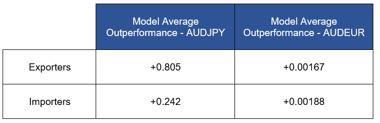
The pattern of results is consistent, with benefits for both exporters and importers.
Why no framework?
This brief study can’t be exhaustive, but to summarise the core questions it answered for us:
Appropriately calibrated frameworks are demonstrably better than the alternative.
Even very basic frameworks can be beneficial.
Proper framework calibration is important before implementation.
In the absence of individual skill (or good fortune), those who operate without reasonable frameworks expose themselves to random or worse outcomes.
This additional ‘cost’ is largely unnecessary and can be avoided.
In the field of investment management frameworks are common and a not onerous to construct. By far a majority of managers typically incorporate them for strategic and/or tactical asset allocations; others include them to distinguish style. Similarly, delegated authorities, limits, and other dealing controls can all be thought of as frameworks. Whether fit for purpose or not, these are designed to enhance performance (and we particularly admire those whose focus is on enhancing risk-adjusted performance).
However, as we have noted before, among the various desk reviews we have conducted there remain areas of activity in which frameworks could be applied or existing frameworks enhanced or reviewed.
Which begs the question – if frameworks can be so easily proven beneficial why not incorporate them in your process or strategy?
At Martialis, we assist clients challenged with building robust frameworks (and reviewing old ones) for decision making under uncertainty. Please feel free to reach out on this topic.
Return to the USD swap pricing basics in a post-LIBOR world

Many of our clients have noticed some pricing differences in basic USD interest rate swaps. The differences were almost entirely in swaps with maturities less than 2 years.
The differences are typically:
During the transition from LIBOR to SOFR, we were regularly seeing the quarterly adjustment spread of 24.8 basis points for the rolls after 30 June 2023. This seemed somewhat strange because the ISDA spread was fixed in March 2021 at 26.161 basis points.
More generally, we see forward-starting swap pricing differing considerably between banks.
The interbank SOFR markets are based on a 2-day settlement delay whereas many corporate trades (to match underlying assets and liabilities) have 2 or 5-day lookbacks. This results in pricing differences especially in steeply inverted rate curves.
This paper uses a simple example to demonstrate how these differences can arise in a pricing model. While this example uses linear interpolation, my testing in cubic spline interpolation gives similar results in the current USD curve.
The maturity model and algorithm
In a LIBOR pricing model, the curve for the first 2 years was typically built from LIBOR and the Eurodollar futures prices. The straight dates (e.g., the quarterly roll dates) for the spot swaps were calculated by interpolating between the implied futures yields and building the curve.
In the SOFR pricing model there is actually a choice. The SOFR markets developed from inputs more related to deposits and loans so shorter dated swaps, say less than 2-years, had basic pillar points from 1 – 12 months and then 18 and 24 months. SOFR futures did not exist when these trading conventions were developed.
As expected, the SOFR swap rates derived from the SOFR futures align with those published on screens with pillar points as described in the previous paragraph. This is unsurprising as the two markets (OTC and futures) are (and should be) very closely connected and are regularly used by many participants.
A rate for a series of one-roll, quarterly swaps can be calculated by interpolating 3-month SOFR OIS and the SOFR futures out to 2 years. The following chart and table shows this calculation based on the closes of 19 June 2023.
The curve is shown in the following chart.

I use the notation of, for example, 0X3 as a one roll swap stating spot and maturing in 3 months. The rates in the following table are derived from those shown in the chart above.

IMM Swaps when spot date is the first IMM date
I notice greater differences in forward start swaps and particularly IMM dates, i.e., swaps rolling on the IMM dates.
If the IMM dates are within a few days of the spot-start swaps, then things line up very well. This can be seen in the following table. In this case, I am assuming the current spot rate is 21 June 2023 to correspond with the June 2023 IMM date.

Note that the rates do differ slightly. This is because IMM dates are not exactly the same as the straight swap dates, so small interpolation differences will be present.
But the rates are generally quite similar and eventually solve to very similar swap rates in columns 3 and 5.
IMM Swaps when spot date is not the first IMM date
This is where the differences become meaningful. I have moved the spot date to 8 May 2023 and kept all the rates the same. This time the rates derived from the swap rates are often quite different to those of the SOFR futures which will not change.
The results are in the following table.

When I move the spot date back to mid-way between IMM dates, the one-roll swap rates and IMM date rates start to differ as seen in columns 2 and 4. Similarly, the maturity swap rates differ as well.
How can this be happening?
The explanation
This effect arises from the fact that the rate curve (as seen in the chart above) is not a smooth curve. It has a few non-linearities (i.e., it is not a straight line) which causes differences if the pillar points of the underlying curve and the swap being priced do not perfectly align.
This is also known as a double interpolation problem. It occurs quite often in swap pricing and is generally exacerbated by ‘bumpy’ input prices from futures when the spot date is between IMM dates.
I also note that the interpolation method is critical. Whether you assume linear, cubic spline or the myriad of more exotic methods, you must understand the positive and negative aspects of interpolation in short-dated swaps where differences are not averaged out over many rolls.
If you ignore the interpolation characteristics (especially for complex methodologies) then you may pay a significant ‘tuition fee’ in a pricing error.
Implications for buy-side firms
The fact that different banks can and do price forward swaps differently means you will likely see different prices for these swaps from banks. While this seems unusual, it is quite expected as they all use different interpolation and pricing methodologies.
Buy-side firms could consider forward-start swaps rather than spot-start swaps. The forward nature of the swap will often create the price differences. The best dates are usually between the IMM dates where most deviations will be maximised
Implications for banks
The golden rule is start with the underlying hedge. If you are using futures, then be aware of a possible double interpolation problem and always revert to using IMM dates to build the curve.
But if you do not use SOFR futures, then price off spot-start swaps and hedge with other banks using the same inputs. You will likely work this out by simply asking for prices and back solving to the pricing methodology.
Summary
There is no ‘absolutely correct’ methodology for pricing swaps with maturities less than 2 years. But all participants should consider:
Where is the start date of the swap relative to the IMM dates.
Whether you use SOFR futures for pricing and hedging. If so, then align the pillar points accordingly.
For buy-side, consider using forward-start swaps to achieve your best price and find the banks with the methodology which will give that outcome.
For banks, consider the hedging strategy and include this in your pricing methodology.
The interpolation method needs to be well understood. All have positive and negative features which should be considered in any short-dates swap price.
Over my many years of pricing and running books, the pricing and management of short-dated swaps is the most complex skill to acquire. Revaluation systems and pricing systems tend to be similar at banks (often the same) so a divergence between the hedging and pricing assumption will not be immediately apparent.
But they will converge at some point and the P&L will reflect the correct or incorrect assumptions.
As always, there is no free lunch.
Execution Costs – Mysterious or manageable?

One of the less well understood areas of finance is the impact of transaction costs on standard risk-reward models. While market makers with deep experience know that transaction size impacts costs, this is often not communicated to end market users in a transparent or quantitative manner.
In this first of a series of pieces, I use the efficient-market hypothesis to examine a number of hedging approaches and their impact on deal outcomes. I will show that averaging can be relatively efficient regardless of transaction size, but also that averaging’s benefits are positively correlated to deal size.
Crucially I use historic data to demonstrate that all-in cost probabilities can be quantified.
The Black-Scholes option pricing model transformed modern finance. Whereas prior to 1973 option prices could only be guesstimated, Black-Scholes presented a ground-breaking framework that birthed standardised pricing.
Coupled with the advent of the personal computer, Black-Scholes changed the manner and speed with which markets calculated risk. While arguments as to the limits of the model abound, elements of the original framework can be readily applied to advance our thinking in other domains.
In this piece I draw on the hotly contested efficient market hypothesis, which posits that market movements are essentially unpredictable, and might be thought of as a 50:50 hypothesis. I have often thought of it as simply that “markets are just as likely to go up, as they are to go down.”
As we shall see, while the hypothesis doesn’t perfectly hold, we can leverage it to assess the efficacy of different dealing execution strategies probabilistically. In this piece I use it to demonstrate that a carefully formulated execution strategy can minimise execution costs.
A market example
Let’s start by defining a simple scenario with key assumptions, of which I have chosen four:
As a hedger we are concerned about adverse market movements in the standard 3-year Australian dollar interest rate swap (IRS) market.
We are worried about adverse movements over the coming 3 months.
We have only two choices of how to execute our hedge:
a. At-Close Risk Cover - a single transaction executed at the end of three months, or
b. Progressive Risk Cover - transacting equal portions daily, accumulating in the outright exposure at the end of three months (i.e., approximately 1/60th hedged per day without exception).
All dealings are conducted at closing rates without execution costs.
I purposely chose the divergent forms of execution since they sit at extreme ends of the hedging spectrum. This is to highlight the importance of hedging strategy and the impact that deal size has on transaction costs.
For the sake of scenario framing, the following chart displays 3-year close-on-close swap yields from February 1991 until May 2023, which has been used in this analysis.

What becomes immediately obvious is that there has been a serial decline in yields (a generally rallying bond market) since 1991. We should remind ourselves that while historic outcomes don’t predict the future, the historic hedging outcomes show serial bias, and this has tended to favour swap payers.
Payers were favoured under At-Close Risk Cover ...
Under At-Close Risk Cover, the hedger is exposed to open market risk through the 3-month period, from initiation to close, with final cover being achieved only at the end-of-period closing price.
If the efficient market hypothesis held, we should expect a broadly 50:50 dispersion of favourable versus adverse outcomes, between payers and receivers.
However, as predicted, the long-term decline in 3-year yields within the dataset skews the outcome in favour of paying hedgers under the At-Close Risk Cover since 1991:
Payers, 53.46%
Receivers, 46.3%
Sum of favourable outcomes, 99.80%
Notice here that I have calculated the sum of favourable outcomes, which seems unnecessary. While this may seem superfluous the sum can be used to illustrate an important point and it gives us our results at base-100 which assists make our key point.
Notice, also, that in the case of At-Close-Cover the results do not precisely sum to 100%. This is because of 8,355 observations; a zero return was found on 17 occasions. On those dates neither payers or receivers obtained an advantage.
…. and Payers were likewise favoured under Progressive Risk Cover.
Under a Progressive Risk Cover model, it is assumed that it is possible to hedge the 3-month/3-year IRS risk at the mid-market daily close in equal daily proportions. This results in an ‘achieved transaction rate’ that is equal to the arithmetic mean of closing rates for sixty trading sessions.
The range of achieved rate outcomes (average rate minus initial rate) should still adhere to the efficient market hypothesis, that is: approximately 50:50 outcome split between payers and receivers.
Again, while our analysis uncovers a favourable bias for payers, it remains fairly close:
Payers 53.96%
Receivers 46.04%
Sum of favourable outcomes, 100.00%
And in this case the sum of favourable outcomes sums neatly to 100%.
What happens when we incorporate execution costs?
The two execution scenarios I have described here rely on the ability of hedgers to transact with perfect efficiency. That is: we’ve assumed hedging can be conducted at market-mid, which is obviously unrealistic.
So, what do we find in more realistic settings?
When transaction costs are included in our analysis, we find three things:
Favourable hedging outcomes are inversely related to transaction size under all execution approaches.
Progressive Risk Cover is more efficient than At-Close Risk Cover regardless of size,
The costs related to At-Close Risk Cover are positively correlated with increased transaction size, both nominally and relative to Progressive Risk Cover.
These findings will be unsurprising to market makers and those with deep markets experience. In fact, those who understand the nature of such costs will be right to ask, so what?
While we have proven the seemingly obvious, the point is:
The magnitude of transaction costs and their impact in large transactions, often fail to be quantitively defined for end users.
And yet there are few reasons for this lack of transparency.
While our experience in this domain would allow us to make reasonable transaction cost estimates, we have conducted soundings with market peers to arrive at indicative spreads.
The following graph collates these estimates of transaction costs and plots the impact they play on efficiency relative (based on 100 being perfectly efficient) to transaction size.

What does this show?
The difference in percentage-favourable results is quite stark.
· The blue line plots the percentage-favourable outcomes under Progressive Risk Cover,
· The red line plots the percentage under At-Close Risk Cover.
What we find is that under all deal size scenarios Progressive Risk Cover outperforms At-Close Risk Cover in terms of transaction costs. And as we noted, deal efficiencies decline as deal size grows for both approaches but maintains near-100 efficiency for Progressive.
Motive Asymmetry?
The field of behavioural finance is strewn with examples of the skewed perspectives found between those who seek to avoid risk and those who actively seek risk for profit. What should be clear is that regardless of motive, transaction costs can alter the standard efficiency paradigm no matter whether you are risk seeking or risk avoiding.
What should also be clear is that how you execute matters, and that the extent of that impact is magnified as deal size grows.
This makes specialist approaches to large or highly complex transactions a must, since a carefully formulated execution strategy can minimise both market risk and execution costs.
What next?
My next blog will focus on the risks associated with different execution approaches, again using progressive versus at-close scenarios and historic data quantitatively. This we will tie in with our work on premium illusion to demonstrate that there really is no such thing as a ‘free lunch’ when it comes to managing risk.
For those who would like to discuss the scenario, its outcomes, and/or the frameworks we use to quantify hedge-efficient approaches, please reach out at: info@martialis.com.au.
The Triennial BIS Survey – USD Derivatives
Every three years I eagerly await the BIS Triennial Survey as it rarely fails to surprise. The 2022 Survey was announced in October 2022 and I have been remiss in not looking into the details of the data.
Hidden in the tables are many interesting facts which correct the market thinking on the state of the FX and derivatives markets, the trends over many years and potentially what to look forward to in the future.
This paper is the first of a series on the 2022 Survey and looks at looks at USD derivatives as was a comparison across the 2010 to 2022 Surveys. I will look more carefully at the 2022 Survey for USD next blog but this will start the process of a longer series on the derivatives markets.
I plan to look at the top 4 currencies (USD, EUR, GBP and AUD) as well as the total market over the next papers.


The USD derivatives market has seen strong growth in average daily turnover (blue line) since the 2007 (i.e., the 2010 Survey which uses data from 2007 – 2010). In fact, the turnover has increased by over 7 times from around 300,000 million to 2,200,000 million per day.
While this is impressive growth, it has not been equal for all market participants.
The Reporting Dealers (orange) have had a moderate decrease in the percentage of the total from 33% to 17% now.
The Other Financials (grey) have increased their share from 54% to 80%.
The Non-Financials (yellow) were never a major component of the turnover but have decreased from a high of 20% in 2013 to around 1% now.

The growth story - Other financials
The growth story (I think unsurprisingly) is the Other Financials, i.e., those who are non-reporting financial firms and typically non-banks.
This group dominates the market with around 80% share of both LIBOR and SOFR markets in the 2022 Survey as shown in the following chart.
This group has grown with the SOFR and LIBOR markets and has largely crowded out other market participant and now represents around 80% of market turnover.
Since 2010, the Other Financials have been well over 50% of the market and have represented the largest group in all the Surveys since 2010. Note that the separate reporting of SOFR started in 2019 and this group has been just as active in SOFR as in LIBOR.

Falling involvement - non-financials
If I then look at the Non-Financials only and compare the percentages of the LIBOR and SOFR markets, the decline of market share for this group is clear in the following chart.
In the Surveys prior to 2019 (when SOFR swaps derivatives were not separately reported), the Non-Financials were not major participants in derivatives. Since 2016, the share of the total (LIBOR and SOFR) has declined.
Since 2019, the share of both LIBOR and SOFR has declined similarly. The Non-Financials appear to be a very small component of the overall derivatives markets in USD.
What could be causing the fall in the Non-Financial percentage?
While it is not clear what caused this decline in percentage, one thought was the interest rate environment.
The following chart shows the Non-Financial percentage and the USD 3-month LIBOR and the USD 5-year LIBOR swap rates. This is to ‘test’ whether the percentage is impacted by the direct or outright short term (LIBOR) or longer-term (5-year swap) rates.

There is no obvious connection between the direction or level of LIBOR/5-tear swap and the percentage for Non-Financials. While the percentage did rise from 2010 to 2016 which corresponded with the fall in interest rates, this was not repeated in the 2019 – 2022 falls in interest rates.
The actual turnover for Non-Financials have been falling as well as the percentage (see the first chart).
Something is happening over the most recent Surveys which indicates the Non-Financials are a relatively small component of the USD derivatives market.
Summary
The trends in the USD derivatives markets can be observed over many years using the BIS Triennial Surveys.
Since the 2010 Survey:
The Other Financials have continued to dominate the USD derivatives market turnover and now represent approximately 80% of the market.
The Reporting Dealers are a declining percentage of the market and now represent approximately 19% of the turnover.
The Non-Financials are showing a multi-year decline in percentage and are now around 1% of the market.
As the USD market transitions to SOFR in its various forms (Term SOFR, compounded and averages) the main users will adopt a standard form of SOFR. The LIBOR reporting will disappear and be replaced by SOFR.
I expect the Other Financials to continue their dominance of the market turnover and potentially increase their share over the next 3 years.
Non-Financials are still a mystery play; will they remain at very low growth levels of turnover or will they return to the markets as rates rise and/or increase in volatility? Will they also adopt SOFR and/or Term SOFR to replace LIBOR or simply hedge in other ways?
My next blog will look further into the USD 2022 Survey for any hints as to how the USD derivatives markets may evolve in the near future.
Variation and Initial Margin Collateral Management - A new challenge
1 September 2022 marked the introduction of the final phase of Uncleared Margin Rules (UMR). This has been a very long process which has included 6 phases and has gradually caused a large number of market participants to post variation and initial margin to support their derivative trading. It is worth noting that UMR only applies to new trades after the date of implementation.
In the case of variation margin (VM), most jurisdictions require ‘financial counterparties’ to exchange VM while generally allowing end users an exemption.
For initial margin (IM), if the Average Aggregated Notional Amount (AANA, which is basically the gross notional of all uncleared derivatives including FX) exceeds a specific amount at each phase, then both counterparties are obliged to post IM for their uncleared non-FX derivatives if they are both ‘covered entities’ (i.e., have exceeded the AANA at any phase).
The implementation calendar is as follows:


Why is VM and IM collateral a challenge?
VM has been used for many years prior to 2017 as a credit mitigant to offset the mark-to-market (MTM) of a derivative with a counterparty. VM can be posted or received depending on the MTM.
IM is posted by both counterparties to independent custodians. It does not depend on the MTM, but rather on the risk of the derivatives. It is seen as insurance against future movements in MTM.
Changes to capital calculations for many banks (Basel I, II and III) have also contributed to the use of VM and IM. Where banks use collateral, they can reduce the capital drag on derivatives substantially, making them more competitive and increasing returns. This impact can also change the pricing of derivatives for end users as banks using lower capital can effectively ‘pass on’ the savings.
While IM Phases 1 – 4 had their own issues, the firms involved had significant resources and experience in managing and providing IM with each other for uncleared exposures and with CCPs for their cleared trades. The problems for these firms were often associated with engaging the independent custodian and setting up separate accounts. For example, in Phase 1 there were approximately 10 firms but they each required thousands of individual accounts at custodians to support the legal entities! All this took time and effort.
As we moved to Phases 5 and 6, the firms captured by the regulations are often less familiar with the operational requirements of posting IM and managing the complexities of posting and receiving VM. They also, like the previous phases, needed to set up custodian relationships and open accounts as necessary.
The number of Phase 5 and 6 counterparties is estimated at 1,200 in total which far exceeds the previous 4 phases (~100 in total). When the significant number of new firms and the probable level of experience of those firms is combined, there are challenges for all participants as there are 2 sides to every transaction with individual and joint responsibilities.
If there is a mismatch in capability and experience between the counterparties, there can be ongoing challenges for both counterparties in both VM and IM.
Challenge 1 – Agreeing and reconciling IM and VM
All regulatory jurisdictions require counterparties to agree the IM and VM amounts daily within quite tight tolerances. If the counterparties cannot agree, then a process of reconciliation commences.
This generally starts with checking the actual portfolio (number of trades) followed by valuations of individual trades (VM) and risk inputs to IM calculations. These activities can be complex, detailed and time-consuming. In many cases, sophisticated quantitative tools are required which may not be readily available to both counterparties. We have found that Phase 5 and 6 firms in particular do not have these tools and processes established and ready to deploy.
With short timelines for reconciliation, some clients are having problems achieving the short turnarounds required for resolving IM and VM differences.
Challenge 2 – Availability of acceptable collateral
Most firms who post or receive VM collateral have reviewed their documentation and restricted the options for that collateral to currencies and/or securities they can access for posting and accept when receiving. For smaller firms, this is often cash in their domestic currency as they have limited availability of foreign cash for posting and limited ability to accept and invest a foreign currency.
Although USD is the standard collateral currency, we have found many smaller, buy-side firms will require their domestic currency as VM. This does solve the operational problem but can create other complexities such as that in Challenge 4.
IM has a very different collection of potential issues. The generally preferred IM collateral is limited to certain types of securities (e.g., government bonds) which are agreed between counterparties and can be accepted by their respective custodians.
Larger firms (banks) can routinely access these securities either directly from their own accounts or via repo markets. Either way, they have established and efficient processes to find and post the required IM collateral.
Smaller firms typically do not enjoy the same access to these securities, especially investors who own other securities aligned with their investment mandates and return metrics. Cash is not preferred by custodians, and they will charge large fees for accepting cash as IM due to regulatory costs. Repo is available but firms still need cash collateral for the repo and the systems and processes to trade and settle the repo. Again, this is very costly and inefficient for smaller firms.
We have found that smaller firms have often had problems accessing and managing collateral especially for IM.
Challenge 3 – Balancing fund returns for investment firms
Investment firms have an additional set of challenges that arise from the multiple funds, legal entities and fiduciary duties associated with those funds.
Many firms need to maintain separation between the funds and accurately record and price collateral borrowed from one fund to post for another fund. This is fast becoming and issue for Phases 5 and 6 firms as they begin to post IM created by derivatives in one fund, but they borrow the securities from another fund. This has to be priced at arms-length and accurate records and accounting entries posted to maintain the integrity of each fund return.
Challenge 4 – Pricing and revaluation
USD collateral is the standard for pricing derivatives and the published prices are assumed to be using this standard. For example, a USD interest rate swap uses USD SOFR as the default collateral as does a USD/JPY or USD/AUD cross-currency swap. In the case of other currencies, the collateral is assumed to be the domestic currency, for example AUD interest rate swaps use AONIA as the assumed collateral return rate.
As outlined in Challenge 2, many smaller firms prefer their domestic currency. In the cross-currency example, many buy-side firms have VM in JPY or AUD depending on their location.
When you change the collateral currency assumption, this can (and often does) have an impact on the price of the derivative. In some cases this difference is small and can be effectively ignored. But in other cases (e.g., cross-currency) the impact can be significant and can change the price.
All firms need to be able to price this difference: either they are charged for it or they need to demand the better price. Otherwise, a sophisticated, unscrupulous counterparty may simply ‘trouser’ the profit and the less aware firm will never notice the difference.
So, what you see on the screen as the price of a derivative for a new trade or a revaluation rate may need to be adjusted for your collateral currency if it is not USD or the assumed domestic currency for that derivative.
Revaluation rates are also problematic for many firms as they must adjust the rate from a screen or valuation service to reflect their collateral arrangements per counterparty. This is very complex and can seriously impact both accounting and the ability to reconcile VM and IM with a counterparty.
Challenge 5 – Back testing the portfolio
Firms included in all IM phases in most jurisdictions are require accreditation by their local, and occasionally offshore, regulatory authority. One of the more difficult and ongoing challenges for many firms is demonstrating appropriate back testing of the portfolio to show the IM posted is adequate to cover the risk of default.
Banks have been doing this for many years with VaR and stress testing requirements. But non-banks have typically not had this form of reporting obligation until they became ‘covered entities’ for IM.
The back testing is usually done daily, and regulators want to see rigor and maturity in testing over a certain period in the recent past and stress tests to cover extraordinary events. This is overly complex and is often a new process for many non-banks.
Our recent work has shown that many firms are finding the technical and operational aspects of back testing difficult to implement. The choice and maintenance of stress events is similarly challenging as it relies on expert judgement to find the appropriate scenarios for their own portfolio.
Summary
Collateral is now part of doing business for many firms, either through regulatory obligation or increasingly through counterparty requirements. Whether using clearing services (i.e., CCPs) or uncleared bilateral relationships, collateral is an important consideration for many firms.
We see the number of firms using collateral increasing and the complexities of managing the operational and technical challenges can be new and significant for many of them. The challenges can be managed with careful planning and some essential tools.
We have listed 5 challenges above but there are often many more. Each firm has their own idiosyncrasies with operational and technical improvements which are needed to manage collateral.
USD Inflation – the barbed wire hedge
Ross Beaney posted a great blog on the Texas hedge which has attracted much interest. Ross provided the definitions for a Texas hedge as:
Oxford Reference Dictionary - The opposite of a hedge, which is intended to reduce risk. In a Texas hedge risk is increased, e.g., by buying more than one financial instrument of the same kind
Collins Online Dictionary - the opposite of a normal hedging operation, in which risk is increased by buying more than one financial instrument of the same kind.
He applied this to the Term RFR and compounded RFR markets to demonstrate the challenges of hedging one with the other.
Today I will look at the barbed wire hedge and I thank Andrew Baume for reminding me of this hedge variant in our LinkedIn post! So, what is a barbed wire hedge?
A definition for this unusual hedge is not available using the usual search methods on the internet because the term probably fell from common use in markets before the internet was ‘a thing’. My last recollection (before Andrew reminded me) was possibly in the early 1990’s and it was described as:
‘A barbed wire hedge is one where it does not matter which leg you lift to extract yourself from the risk and/or hedge, you are in trouble!’
The picture tells it all……….
In this blog, I look at the USD inflation markets and how the barbed wire hedge is an apt description for the challenges faced by many hedgers and the dealers who provide the prices.

Inflation history
The following chart is for the annual inflation printed in USD over the past 10 years. I use the annual data because it removes the considerable seasonal variations in US CPI and focusses on the actual trend.

There has been little or no trend until 2020/21. Everyone has noticed the increase in inflation in 2021 and 2022 which is clear in the chart above. We have had relatively low inflation for many years which has been broadly in at the Fed target of 2%. This can be seen in the next chart showing annual inflation outcomes since 1960 where inflation since 1995 has moved in a band between 0% and 4% oscillating around 2%.

But now we are close to 5% and trending up. Interest rates aside, what should we do to directly hedge our inflation risk? Will inflation peak this year as many expect? Or will inflation become more entrenched as we see happened from the mid-1970s to the mid-1980s?
I will not cover the possible causes for higher inflation in this blog but rather look at the challenges for hedging and what this can mean for hedgers and dealers.
Looking forward and inflation expectations
The following chart shows the 10-year forward USD inflation expectations over the past 10 years.

The markets clearly expected 10-year inflation averages to be around the 2% target until the COVID19 drop in early 2020 to a low around 0.5%. This quickly reversed as markets expected the US market to recover more quickly and priced in higher inflation.
The next chart shows the current, implied forward USD inflation rates (annually) for the next 10 years. The 10-year inflation swap is around 2.7% which incorporates the current expectation at 5.38% but the forward rates fall rapidly to 2% - 3% in subsequent years.

Markets are very clearly pricing a very transitory period of inflation followed by more ‘normal’ inflation rates around 2% after 2023/24.
The hedge challenge – the classic barbed wire hedge
With current inflation rates higher than in the past 20 plus years and seemingly trending up, there is an immediate decision for many firms to consider hedging. Or not.
Now, you are metaphorically astride the barbed wire fence. You hedge now and you lock in inflation at an average of 2.7% for 10 years with the implied rates in the previous chart. While this looks attractive, what if there is a recession and inflation returns to near 0% as it did in 2009 and 2020?
Or you could wait and see.
This also comes with a risk of a repeat of the mid-1970s to mid-1980s where inflation ranged from 5% to 14%.
Which leg do I lift first? Do I lift the hedge leg and accept the risk of higher inflation? Or do I lift the risk leg and lock in the current inflation curve? This is a classic barbed wire hedge conundrum where whichever decision you take, there are consequences, and you may wind up in trouble.
Summary
Decisions come with risks, but decisions must be made. The way forward for inflation is not as clear as it has been for many previous years where we had inflation expectations and outcomes around the 2% target. The current expectation is a return to the benign world of approximately 2% in the next year or so. But this may not be the case.
Whether you decide to hedge or not and whichever leg you decide to lift, there may be a time when you quickly need to reverse direction and replace the leg you lifted. To continue the analogy, when you are captured by a barbed wire hedge, take careful note of which leg to lift, manage the risks during and after the operation and be prepared to reverse if things start to go badly wrong.
Otherwise, the outcomes can be painful.
Of Texas Hedges
Questions around use case limits for Term-RFR rates have been raised many times, and we devoted some attention to this topic in my most recent Blog; but whatever policy firms decide upon, there is one very real and practical reason why firms should carefully think about their use.
In this blog I take a look at the question of whether traditional overnight index swap products should be used to hedge term deals? Those with deep derivatives experience should already be aware of this problem since it already arises when LIBOR and OIS products and risk interacts.

Texas Hedges
Most people in finance have heard the expression “a Texas Hedge” without having unduly bothered with a proper definition of the term. Is it a hedge that works only partially? One with known or unknown risk gaps? Is it somewhat ‘cheaper’ than a traditional hedge?
I had always assumed it was a hedge that was unlikely to work as the hedger intended; a kind of Saguaro Cacti where topiary would have been more appropriate! It turns out that I was quite wrong. If you thought likewise, you probably weren’t alone; but you were also wrong.
To share some easily available definitions is reasonably instructive:
Oxford Reference Dictionary - The opposite of a hedge, which is intended to reduce risk. In a Texas hedge risk is increased, e.g., by buying more than one financial instrument of the same kind
Collins Online Dictionary - the opposite of a normal hedging operation, in which risk is increased by buying more than one financial instrument of the same kind.
And while we are loathe to resort to Wikipedia, it does fall into line, defining a Texas Hedge thus: a financial hedge that increases exposure to risk.
Whatever the understanding, most people simply recognise that the term is typically used in the pejorative, i.e., they’re a bad idea.
In BOTH the old LIBOR world and in the post-LIBOR world, there was and is an inadvertent Texas hedge problem that emerges when one attempts to hedge term-rate deals with common overnight index swap products (OIS), and it’s a problem that meets the definitions outlined above; that is, when standard OIS are used to hedge term deals risk is actually increased.
A bifurcated derivatives market (term v OIS)
We have written about the emerging benchmark landscape several times in the past year. This is because it is creating variability and choice in both corporate finance and across the derivatives space. We have also looked at the problem of the basis, liquidity, operational and accounting risk that can emerge when deals and hedges are not like-for-like matched on a benchmark and/or convention basis.
I don’t propose to delve further into any of these topics here, except to point out that where term products (cash or derivative) are hedged with non-term equivalents, basis, liquidity, and operational risk can and typically will, arise. And while we don’t wish to downplay these risks, they are somewhat unlikely to be the biggest risks faced.
While there is an emerging smorgasbord of underlying benchmarks (and thus choice), the risk of Texas hedges emerges when participants attempt to hedge products referencing the emerging suite of term rates, whether in cash or derivative products, with standard OIS derivatives.
In fact, this risk was around well before LIBOR reform ensured it would be revisited; OIS hedges for LIBOR risk have long been known to pose the same issue that I will outline here. The problem has come to greater prominence in the post-LIBOR world because the emerging benchmark choices have created a degree of confusion (and in some cases inertia), and use-case limits may restrict the availability of hedges in ways that were (to us) likely unintended.
I will now turn to explaining the peculiar risk that arises.
Bigger than basis
Imagine a simple situation in which a borrower has chosen to borrow floating under the terms a facility that references a 90-day Term-RFR as distinct from daily compounded or simple RFR. The underlying currency and RFR is quite irrelevant.
The mechanics of the reset feature under Term-RFR are analogous with that which operated under LIBOR, and I will represent the reset risk with individual arrows (rather than traditional swap flow diagrams) to keep things simple:

In this simple example, let us assume that Party-A has an initial risk profile whereby they receive floating rate payments based on a Term-RFR benchmark from some undefined cash instrument at 90-day intervals for one year.
The initial reset, (r1), is the only known reset at the outset. The remaining rates, (r2-4) are all unknown, though market makers can readily imply (price) them if desired/required.
What happens in practical terms when these floating rate receipts are ‘swapped’ for a fixed rate?
Very simply, Party-A agrees to pay floating (the lightly shaded red arrows below), in exchange for the floating receipts (the blue arrows) and in return for this swap they receive a fixed coupon at each payment date. We will denote the fix at a rate of RFIX.
The rates used on both sides of the floating risk produce precisely off-setting payments

But what happens if Party-A is receiving floating payments from a Term-RFR cash instrument? Can they use an RFR referencing OIS hedge to transform their exposure to a fixed rate in the same manner as Diagram 2?

The answer is no, at least not perfectly, and there is a big catch that people need to understand.

The fundamental problem here is well known to professional market derivatives experts; a known forward-looking cashflow reset at R1, is exceedingly unlikely (except by chance) to match an uncertain back-wards looking OIS payment which can only be calculated in arrears (r?). If these did match, every OIS traded would settle with zero cashflows.
Aside from an inability to cashflow match (which introduces basis risk), each progressive OIS stub of the OIS hedge becomes problematic in ways that are not immediately obvious. To make this more obvious, let me use a simple hypothetical scenario to make it clear.
Under a traditional like-for-like swap there is no slippage on either side of the floating rate payment schedule; the fixed rate outcome of the swap is assured:

Note that all the rates here are fictional, not some current or past yield curve.
Under OIS versus Term-Rate there is the potential for theoretically unlimited slippage or gain on the OIS side of the payment schedule.
To keep with simplicity, I will assume that the OIS in-arrears payment made under the terms of the OIS swap is 100 BP higher than that of the fictional term rate. This might be based on a shock market occurrence that appeared after the first reset.

Keeping with simple (I.e., no discounted cashflow) maths, it becomes clear that if simple RFR rates (overnight rates) were to RISE dramatically, the payment required under the floating leg of the OIS hedge (‘hedge’) rises, thus LOWERING the effective received rate of Party A.
The result contradicts Party-A's intended strategy (yield maximisation).
This meets a formal definition of a Texas Hedge
And while I did not expect this simple blog to result in finding a genuine textbook Texas Hedge, it seems we have. The mismatch between hedge and hedged item has INCREASED risk.
Implications?
What are the implications of all of this? Some basic directions seem most appropriate:
For parties that do not run trading books that are able to warehouse such risk:
Understand your underlying benchmark – e.g., is it fit for your purpose unhedged?
Understand the product-type and its relationship with the benchmark.
Understand the use-case limits that might restrict your freedom to engage firms to hedge, and to unwind hedges at some point when doing so might be advantageous,
Adopt a like-for-like approach to hedge versus hedged instrument where possible,
Discuss what you’re doing with audit to gain an understanding of their views on accounting treatment.
For service providers:
Ensure your teams understand the emerging smorgasbord of benchmarks,
Consider the boundaries of your product suite; a too narrow suite can be problematic,
o If your corporate finance team is doing term rate deals your customers will surely require like-for-like hedges?
Develop use-case policies that meet the various licencing and regulatory expectations,
Take steps to ensure relevant staff understand the dangers of recommending mis-hedging to clients based on a failure to appreciate the important differences between products and the mechanics of how their cashflows are determined.
Or at least put up a big sign in your treasury office – NO TEXAS HEDGING!
Cross currency basics – Hedging options for dealers
In previous blogs I have looked at cross-currency swaps from the position of the end-users. In this blog, I will look at a critical change to the way in which the dealers have to operate since the markets switched to being SOFR-based.
Why does this matter? It matters a great deal because the potential, added costs associated with the new hedging options can become significant and change the pricing for end-users. Every basis point of cost needs to be recouped in some way and this can result in wider spreads for buy-side firms. Looking at the options available for dealers can help explain why this can happen and why additional spreads may actually be unavoidable.

The current markets
Let’s start with two typical markets in cross-currency: AUD and JPY versus USD.

In these examples, the USD side is SOFR, the AUD is BBSW and the JPY is TONA which are the current inter-dealer conventions.
The curves are quite clearly shaped and reflect the market flows I have previously described in my first blog on this topic. The AUD curve is interesting as it definitely shows the flow direction out to 20 years is for end-users to ‘borrow’ the AUD leg (i.e., swapping USD debt for AUD). This then dips down at 30 years where opposing flows (long-dated FX options) take the margin into negative territory.
The JPY curve is the opposite driven by end-users looking to swap USD investments to JPY.
The way things were (pre-September 2021)
In the ‘good old days’ when the role of the cross-currency dealer was based on the old conventions, the management of their books was a well-oiled and efficient process and the pricing to the buy-side reflected this situation.
So how did it work in the AUD/USD example?
Each rollover, the USD and AUD were rate set from LIBOR and BBSW, typically 3-month. (In this example, I will use Term SOFR to replace LIBOR so the curves still match.)
At the start of the relevant period, the Term SOFR and BBSW rate sets as well as the 3-month forward FX were all known, and the dealer could calculate the implied BBSW rate from the spot, 3-month forward FX and the Term SOFR. Using these inputs, we can see the calculations in the following table.

If the dealer had received the AUD/USD 5-year cross-currency swap at 6.5 basis points from a buy-side USD borrower (as described previously and from the chart above), the dealer could roll the position at -25 basis points in the 3-month and benefit 31.5 basis points from the curve shape for that rollover.
While this looks like an arbitrage, in reality the dealer is accepting the short-term rollover risk rather than hedging the swap with another 5-year swap. This technique is quite common among the dealer community and is critical in managing a book profitably. The FX spot, forward and rate sets risks offset, and the dealer is square for that roll.
Note the direction: the 5-year swap had the dealer short AUD spot which has to be rolled forward by a buy spot/sell forward 3-month FX swap. This is the equivalent of the dealer borrowing the AUD short and lending it long creating the maturity mismatch.
What happens now?
Staying with the AUD/USD example, the situation is now different because the USD refixes every day and compounds daily rather than fixes once at the start of the period.
What is the dealer to do? They could:
Lock in the USD rate with a 3-month OIS (Overnight Index Swap) and roll the FX 3 months as before. This would attract a spread as the dealer enters the OIS market and pays the OIS trader for the risk.
Roll the FX 3-months to offset the BBSW rate risk and let the USD float for the 3 months. This is cheaper but does leave the dealer with an unhedged USD 3-month rate set risk which they created from the 3-month FX forward.
Roll the FX O/N to offset the USD rate set risk and transact an AUD OIS to offset the BBSW rate set risk. This is unbelievably expensive: the AUD OIS spread is present as in point 1 but it is dwarfed by the implied interest rate spreads in O/N AUD/USD which can be 25 basis points from mid to bid/offer! This is the last resort.
Whichever way the dealer choses to proceed there is residual risk or a new spread to be paid. This additional risk or spread will have to be reflected in the original 5-year swap quote to the end-user.
The JPY example
In JPY we have the opposite side to the trade, but the challenges are essentially the same.

If the dealer had paid the JPY/USD 5-year cross-currency swap at -73.375 basis points from a buy-side USD investor (as described previously and in the chart above), the dealer could roll the position at -33.77 basis points in the 3-month and benefit 39.7 basis points from the curve shape for that rollover.
As we can see, the shape of the cross-currency basis curve is again typically in favour of the dealer rolling short-term and trading with end-users in the longer dates.
The options for the dealer are similar to the AUD example except both sides of the swap are now compounding rates.
So, we have:
Lock in the USD and JPY rates with a 3-month OIS and roll the FX 3 months as before. This would attract 2 new spreads as the dealer enters the OIS market and pays the OIS traders for the risk.
Roll the FX O/N to offset the USD and JPY rate set risk. This is again prohibitively expensive because the implied interest rate spreads in O/N USD/JPY are also very wide and costly. This, again, is the last resort.
Summary
The cross-currency markets have changed and have created new challenges for cross-currency dealers. Whichever option they take to roll their positions forward in the FX market they attract new spreads and costs.
These new risks and costs will have to be reflected in the pricing for end-users.
Cross currency basics 6 – Revaluation of trades
In this sixth instalment of my series on cross-currency swaps I look at how the changes to market inputs for cross-currency swaps have impacted revaluations since December 2021. Previously, I have looked at pricing of cross-currency trades and this blog extends those concepts to revaluation.
Many of our clients and contacts have fixed USD legs on their cross-currency swaps and as a result, they were not required to make extensive changes to derivative contracts to accommodate the cessation of LIBOR since these deals do not directly reference USD LIBOR. While this is quite correct for the contractual matters, many are now finding the revaluation of these derivatives is no longer accurate.
How could this happen? The trade is fixed USD so there should be no problem with revaluations. However there is a problem, and it needs to be addressed.
Let’s look at the causes and possible solutions.

Possible cause - system revaluation inputs
All booking and revaluation systems require inputs to build the necessary curves and valuation rates for cross-currency swaps. These inputs are very precisely defined and include:
single currency interest rate curves which have a particular day count and frequency on the fixed leg (e.g., 30/360 semi, act/365 quarterly);
cross-currency basis curves (e.g., USD LIBOR/AUD BBSW, USD LIBOR/EURIBOR); and
spot FX rates (e.g., AUD/USD, EUR/USD).
The cause of the revaluation issue is often due to the details of the inputs having changed in the data sources while the revaluation system is still using the current definitions. This causes a significant mismatch, and, in many cases, the mismatch will create havoc in the revaluations!
Some current examples of changes to inputs
As markets transition from LIBOR to other rates, the published curves will change. In some cases, the data source (e.g., Bloomberg) will attempt to derive a synthetic version of the LIBOR rates for continuity, but this is not always the case. And even if the derived LIBORs are available now, there is no guarantee they will always be available.
I have taken a few examples in the following table for a five-year maturity swap with some typical rate inputs.

As you can see, the old and new rates are very different.
Why does this matter?
The changes can be problematic if the data sources used by your revaluation system are collecting the new rates and applying them to the existing input definitions. For example, if your system is configured for USD with LIBOR (old input) and you are now collecting SOFR (new input), the revaluation rate could be 28 basis points different.
Similarly, the AUD/USD cross-currency basis could be 26 basis points different if you are using the current, published basis curves but applying them to the existing definitions in the system.
This mismatch can and does cause many of the current revaluation differences for our clients.
The possible solutions
We recommend the following solutions to this problem:
change the system configuration to the new inputs (preferred); or
modify the new data inputs to create derived inputs for your system (less preferred).
Solution 1 - change the system configuration
Where possible, the neatest and most reliable solution is to ‘raise the hood’ on the revaluation system and start to adjust the settings. This may be as simple as setting up new curves with the new input definitions and allowing the system to sort out the details. But it can also be problematic and challenging without vendor assistance.
While this looks attractive, many systems were not designed for this activity and could require considerable adjustment to assemble the required basis curves (e.g., USD LIBOR/SOFR) to transform the new rate inputs to the required rates for all the currencies.
In the USD case, the fixed rate may be valued from LIBOR-based curves now but SOFR-based when you make the changes. This could amount to 28 basis points which will create a USD value. The cross-currency basis will adjust for this change, but the revaluation offset to the USD difference is on the non-USD side because the cross-currency spread is adjusted on that side.
These changes can have quite significant revaluation impacts and care is required to set up all the new curves and ensure the appropriate basis curves (e.g., USD LIBOR/SOFR) are correctly used to minimise the disruption. But if it is done correctly, this solution can be quite robust.
Solution 2 - modify the new data to create the derived inputs
While this is not our preferred option it is often the only solution if your system cannot be changed to accommodate the new inputs.
In this case, the new inputs are entered into another system (e.g., spreadsheet) and the required inputs for the revaluation system are calculated and then entered each day as usual.
The key issues with this approach are the construction and maintenance of the spreadsheet. The algorithms will need to be prepared and entered to the spreadsheet, and this needs to be maintained for the inevitable errors during the life of the trades.
This approach is also problematic for new trades attached to the new trading conventions which are moving from LIBOR. You may need 2 sets of curves: one for the legacy trades and one for the new trades.
Summary
This is a real and current concern for many firms. Incorrect revaluations can be very frustrating and problematic for accounting accuracy and possible collateral calculations (if required). Significant errors can arise if the inputs and curve configurations in systems are not exactly aligned. Firms should also consider the possible accounting and regulatory implications of revaluation errors.
There are at least 2 workable solutions, but both require expert attention. Adjusting or changing the revaluation system is preferred but sometime this is not possible, and it can be impractical. In that case, the only real option is to create another system to transform the new inputs into the system-required inputs.
Martialis is actively supporting our clients in pricing generally and in cross-currency. We see these issues regularly, but they are quite solvable with some dedicated assistance.
The nature of premium illusion in finance – Part II
I noted in my last blog that I intend to write a series of blogs that examine premium illusion, describing it as an issue that market risk decision-makers may not realise they even encounter.
Premium illusion is a related topic within the field of financial loss aversion, which has been studied extensively, and which holds that it is basically natural to have a heightened sensitivity to losses versus gains. However, the not unnatural fear of financial loss from the paying of option premiums is quite chronic, but can be found to be unwarranted (illusory).
In this blog I’m going to turn from a market in which I knew (well, in truth I suspected) there would be solid evidence of illusion, to one that I don’t: the Foreign Exchange market.
I’m surprised by what I find with this rather simple analysis. I suspect readers will be too.

Premium illusion defined
In my last blog I did a rather poor job of explaining premium illusion.
Readers should note that the work presented here is predicated on my personal definitions, formed after having worked in markets for financial options for many years. They should also be aware that I have at times been a very heavy user of financial options and a serial payer of option premiums in various dealing settings.
Of definitions, there are plenty of obscure and some better-known financial texts that contain different definitions to my own. What’s important is not necessarily the neatness of the definition, but what readers are able to make of the data analysis presented in this piece.
With those caveats out of the way, I want to try and clear up a key distinction; while premium illusion is related to premium aversion, there are subtle differences in the financial markets’ product context. This is particularly the case where market participants consider the use of option products versus what we might call ‘non-premium’ products:
Premium aversion is the desire or preference to avoid paying premiums, regardless of the assessed value of an option holding in a particular risk setting,
Premium illusion is a mistake of premium value-interpretation and comes in two forms:
the impression that premium expenses are almost certainly irrecoverable, or typically worthless; and
the impression that non-premium instruments are ‘free’ or contain no potential future premium in the form of opportunity, or actual loss.
I should also mention that while option products are somewhat similar to insurance products, there are key differences, which is perhaps a topic for another blog. What readers should note is that typical price-setting frameworks for financial options consists of professional, two-way markets, where premium payers and earners trade freely with each other in increasingly transparent markets for implied volatility (that crucial common determinant of options value).
A crazy way to assess option value?
In keeping with the approach to assessing options value of my first blog, I look at value in a comparative setting between competing products, one containing an up-front premium, and one that does not. Readers will recall that I make no attempt to conduct an assessment of whether premiums paid resulted in positive option pay-offs at expiry.
Why?
Because the terminal pay-off approach can be quite misleading where risk-hedging is concerned. Also, studies of terminal payoffs have been done many times elsewhere, and of course such studies tend to show that options have a chronic tendency to expire worthless (another potentially misleading result and another possible future blog topic); our task here is to demonstrate whether there is a genuine value to holding intertemporal choice!
My approach is very simple. To recap:
Assume you are tasked with hedging a future short exposure to the AUD/USD exchange rate with a 1-Year horizon (i.e., typical of an Australian exporter)
Your mandate requires that you must hedge, but you’re left free to choose between:
entering a 1-Year forward purchase (i.e., hedging fixed)
buying a 1-Year call option to the forward expiry
Here, I exclude the choice of doing nothing for the reason that I am wanting to demonstrate premium illusion between competing financial markets products (doing nothing is certainly a valid strategy, but it does not involve competing products).
Data selection?
While it may be instructive to look at randomly selected data, and this may become a topic for a future blog post, in this study I am simply using ten years of AUD/USD FX data up to February 2022, comprising:
Outright Spot
1-year Forward
1-Year at-the-money forward call premium
There is nothing particularly special, and certainly nothing random about ten years (2,368 observations) of AUD/USD FX data. It is, however, topical for local and some international currency hedgers, and I hope to be able to show some serial features of premium illusion that local readers will be familiar with.
Why only 2,368 points in ten years? A typical market standard of options users is to apply a 262-trading day approach to annualization. However, while we have ten years of historic spot data, we only have nine full years of outcomes.
What are we looking for in the data?
This is the simple bit; we are asking the following question in 2,368 trials of call option outcomes versus outright-long forwards:
How often did subsequent SPOT fall below FORWARD minus CALL premium prior to expiry?
That is, having purchased a CALL option for a premium of X, how often did SPOT AUD/USD market subsequently move to a more favourable level below the outright forward adjusted for the up-front cost (X) of the option.
More favourable level? Yes, that’s the level where the hedger can purchase (and swap forward) at a rate more favourable than the prevailing forward. It’s typically referred to as the break-even level, but we have to be careful with that terminology in the context I am using it (since it typically refers to in-the-money break-even).
What are we ignoring?
The framework I’m using here is extremely basic; ignoring elements of potential options value that are particularly hard to assess.
A more robust study, including residual options values, requires a serious data analysis package and ten years of option ‘volatility surface’ data, thus making it a very large computing challenge. This may also become a topic of interest for us in future blogs, where we will be able to more fully demonstrate illusion.
What’s important to note is that the analysis presented below will certainly understate the full extent of premium value, and therefore the illusion in the AUD/USD market for CALL positions. This is for two reasons:
I make no attempt to estimate the extent of residual premium one could recoup by selling back purchased options when favourable spot levels present (wildly underestimating the value of the options strategy).
Likewise, I make no attempt to asses the extent of forward-rate conditions when spot falls to favourable levels, which given the fact that AUD typically trades at a forward discount to USD are likely to be quite advantageous (all-bar 31% of the observations in the data here).
However, notwithstanding the extent to which my basic analysis underestimates the potential value of optionality or intertemporal choice, value is still quite clearly indicated.
How often did a 1-Year CALL present greater value than a forward?
I mentioned in the introduction that even I was surprised by the results of this analysis.
Why?
Because I was unsure what it would show (there’s that randomness), and the results suggest there is a consistent advantage. Consider the following:

To interpret this, think of the results at each end of the spectrum shown here:
41.3% of the time a call option strategy outperformed a forward hedge within 3-months of its purchase date.
75.8% of the time a call option outperformed a forward hedge at some point in its comparable life.
Within 6 months of purchase, at some point, the option product typically outperformed the forward hedge (by quite a robust margin – above 60% of the time).
What the data is not saying?
It’s important to note that the question I asked of the data was how OFTEN did the call strategy beat the forward, not HOW MUCH did it beat it by. That is; I make no attempt to determine the average value gained when the option strategy pays off, since such an analysis would be too cumbersome and require too many forced assumptions to be viable (though I may take a shot at this in the future).
It’s also important to judge potential gains versus the average option premium paid to engage the CALL strategy. This averaged 0.03035 (303.5 USD pips per AUD) over the ten years, which is the average loss relative to the forward when the CALL strategy failed (i.e., 24.2% of the time).
As an early lecturer once made abundantly clear: there is no free lunch with options.
An example
By way of exemplifying the potential value I selected a single random date where there was a positive CALL outcome relative to the forward: 15th February, 2018.
Sticking with our simple hedger-example, we assume that on this day the choice of hedge for a 1-Year exposure is between:
A: An OUTRIGHT FORWARD at 0.79623
B: A CALL Option struck at 0.79623, costing 0.02605
The CALL can only potentially outperform the OUTRIGHT FORWARD if spot falls below 0.77018 (i.e., 0.79623 less 0.02605) at some point is the 12 months prior to expiry of the option.

Which is suggestive of a significant outperformance of the CALL in this single sample.
If we add in a rebate for the sell-back of the remaining CALL option value on three dates (3, 6, and 9 months respectively), the relative outperformance of the CALL can be calculated.

What about PUTS?
At this point it is reasonable to ask: Would PUT options analysis of the same data-set show similar results if we assume the hedge required were to protect against a falling AUD/USD rate.
It turns out that the results for PUTS are not wildly different to CALLS:

In other words, it hasn’t mattered whether we are looking at up-side or down-side hedges, option products appear to have a strong tendency to present favourable hedge outcomes in the historic data.
Is this sufficient to confirm premium Illusion?
The evidence of favourable relative value outlined here is quite strong, perhaps surprising, but is it sufficient to confirm widespread premium illusion?
The answer is no, not in isolation.
In an attempt to confirm the evidence of premium illusion I turned once more to Bank for International Settlements BIS data, which shows (as it did for IR-Swap versus Swaption data) that options use is far outweighed by that of outright spot/forward in product usage:

In other words, FX Spot/Forward product use appears to run at a factor approaching 7-times (6.8x) that of comparable FX-Options products, despite evidence of more balanced value outcomes between the competing products (and this despite the fact that the bulk of FX Options turnover is interdealer driven – approximately 3-1x).
Which suggests there is something fundamental that deters hedgers from deploying option products within hedge programs.
That something is likely to be premium illusion mixed with an overabundance of outright premium aversion.
Cross currency basics 5 – Portfolio versus individual deal hedging
This is the fifth instalment of my series on cross-currency swaps. Previous articles have covered the basics, looked at some pricing aspects and the revaluation challenges brought about by changing conventions and some examples of how cross-currency swaps are priced in practice.
In this blog I will look at how the portfolio and individual deal hedging works and some of the challenges for end-users.

Firstly a few definitions:
1) Portfolio hedging
Some firms, such as investment funds, have a number of portfolio managers and currencies where returns have to be converted back to the domestic currency. Other firms, such as corporates, may have revenue and costs in different currencies which likewise must be managed and/or converted to their domestic currency.
Some of these firms use a portfolio hedging approach where they broadly manage the risks and cashflows with a few cross-currency swaps and separately manage the cashflow mismatches with short-term products such as forward FX.
The following diagram shows this approach for EUR and JPY exposures swapped with two cross-currency swaps to USD.

1) Individual deal hedging
Another way to manage the currency exposures is to exactly match each risk with a specific cross-currency swap which converts each cashflow into the domestic currency. The aim is to minimise the mismatches and remove any currency risk from cashflows.
The following diagram shows this approach for the same EUR and JPY exposures but individually swapped with six cross-currency swaps to USD.

Portfolio and individual deal hedging each has benefits and challenges which need to be carefully considered before trading and also during the lifetime of the trade.
Portfolio hedging
This approach uses an overlay technique to provide a broadly-based hedge rather than look at individual risks. It is often used by larger firms who consolidate their currency hedging into a single desk. For example:
Large investment firms often use a mix of external and internal fund managers to spread risk and returns across currencies and management styles. This can result in many currency exposures which need to be converted to the domestic currency.
Large corporates can have a variety of debt and revenue exposures across currencies and maturities. This leads to a complex exposure where they need to balance the assets and liabilities per currency and ultimately back to the domestic currency
In these examples, the number of exposures and currencies can make a portfolio approach more efficient and easier to manage both operationally and for risk.
Benefits and challenges of portfolio hedging
Benefits include:
The number of trades is reduced, often resulting in more tractable system and process management.
The number of settlements is also reduced which can save on operational costs and reconciliation processes.
Challenges include:
The exposures are only approximately hedged which can lead to cashflow mismatches and tracking differences.
Accounting treatment can be complex (hedge effectiveness tests).
Short-term cashflow differences need to be managed with other products such as forward FX which can lead to additional costs and complexities (more on this in a later blog).
The maturity of the cross-currency swaps may not match the underlying risks leading to the potential for over or under hedging.
Allocation of the costs and benefits to each portfolio can be challenging.
Individual deal hedging
This approach exactly matches each exposure with a cross-currency swap. Many firms, especially ones with limited exposures to other currencies adopt this technique. For example:
Investment firms with only a few offshore investments tied to specific assets with known returns and maturities.
Corporates with offshore debt issues and domestic assets that the funding is directly supporting.
Individual deal hedging is attractive to many firms but, like portfolio hedging, has benefits and challenges.
Benefits and challenges of individual deal hedging
Benefits include:
The cross-currency trades will match the underlying exposure and the cashflows will net in the non-domestic currency thereby reducing the need for additional cash management.
Accounting can be simplified with the one-to-one match.
Challenges include:
The number of trades could be significant leading to additional system and process requirements to manage the settlements and reporting requirements.
This is not scalable – it is only effective for a relatively small number of exposures.
Which approach is better?
There is no answer for this question: it all depends on your circumstances. However, there are a few basic inputs to any decision:
How many exposures do I have or are likely to have? A small number may mean the individual deal rather than the portfolio approach as a more efficient and appropriate solution.
How sophisticated is my trading capacity? The portfolio approach assumes a high level of trade management and ability to successfully manage many settlement mismatches in various currencies.
How will my systems and processes manage? A large number of trades, which may result from the individual deal approach, may require advanced systems and processes. The potentially smaller number of trades in the portfolio approach can simplify the swaps but may complicate the forward FX management.
Do I have specific accounting and reporting requirements? This is definitely a consideration as it may favour one approach over the other.
Could I use both approaches? Yes, this is possible and may actually suit many firms with segregated businesses and/or exposures. For example, a single debt issue may be individually hedged but revenues may use the portfolio technique to better advantage.
As I said above, it all depends.
Summary
There is no simple way to approach the complex task of swapping non-domestic currencies to the domestic currency. Every firm with an exposure will have to manage the cashflows in some way and this is often done with cross-currency swaps.
It is vital to assess your operational and risk management capacity to make a decision. A recent blog by Ross Beaney about the need for clear frameworks is very applicable here. Without an honest assessment of your capabilities and an agreed framework for any actions, there is a real probability of a sub-optimal (i.e., disastrous) outcome.
A thorough analysis of your capabilities and exposures is a great start, or a great review of a current process. We have done this many times and really recommend a structured approach to minimise the risk of operational mayhem and/or pricing errors.