Derivatives and USD Term Rates

This article continues the series on the practical uses of term risk free rates (Term RFRs) in USD. Previously, Ross and myself have both looked at the USD term rates where we are seeing significant interest in Ameribor, AXI, BSBY, Term SOFR, CRITS and CRITR. They all have uses and many market participants are actively looking at the way these new reference rates can complement[RB1]  compounded SOFR and provide a more appropriate solution to their requirements.

In this article I look at derivatives and how these important hedge products are being introduced into markets referencing the term rates.

Derivatives referencing compounded SOFR

The market for interest rate swaps and cross-currency swaps referencing compounding SOFR is well established now and supported by price-makers and some end users.

However, the basis swap market is still developing with some swap pairs liquid while others are less so. Examples with significant liquidity include:

1. USD LIBOR/SOFR; and

2. Fed Funds/SOFR.

Some examples of developing markets with identifiable pricing include:

1. BSBY/SOFR; and

2. Ameribor/SOFR.

Other reference rates such as AXI, CRITS and CRITR have some pricing transparency, but it has been somewhat more difficult to quantify at this early stage.

Basis swaps are not static and can vary considerably. The chart below shows the last 11 months (since BSBY has been available) of the USD SOFR versus other reference rates. Since there is some volatility (noting Fed Funds is on the secondary axis) many users may wish to hedge the exposure!

Basis swap markets are essential and provide different market participants the ability to transform their current risks to something more appropriate. For example, the combination of a fixed-rate debt issue by a corporate could be converted to and Ameribor reference by a combination of a Fixed rate to SOFR swap and a SOFR to Ameribor basis swap.

Of course, this can be delivered by a bank in a single swap, but the pricing would typically use the combination if a fixed swap and a basis swap to achieve the outcome for the corporate and a hedge in the inter-dealer market.

Derivatives referencing Term SOFR

Derivatives referencing Term SOFR are available for end-users. An active and available derivatives markets is essential to provide effective hedges for loans, debt issues and investments.

But there is a catch: the inter-dealer market for Term SOFR derivatives does not yet exist. Risk.net has a great article on this problem titled ‘Term SOFR restrictions spark valuation debate’. The Fed and ARRC guidelines restrict the use of Term SOFR derivatives and effectively do not allow inter-dealer trades.

This means dealer books can be one-way with the end-holders and there is no way to clear this risk in a similar way to other derivatives: i.e., hedging with other dealers with opposite positions or views.

There are no on-screen prices, so dealers are obliged to use internal models to replicate the valuation curves. While this is somewhat trivial (with the Term SOFR and compounded SOFR forward curves theoretically identical) there can be small differences due to hedging, collateral and one-way adjustments which need to be considered when building the curves.

In addition, if Term SOFR derivatives cannot be identically hedged then they may be consigned to the ‘structured’ book within the dealer firm and attract additional reserves and capital.

Either way, the absence of the interdealer market is very real and has consequences for all market participants who may use these derivatives. 

Why does the absence of an inter-dealer Term SOFR derivatives market matter to end-users?

It matters for at least 2 reasons: cost and availability.

Firstly, dealer costs would very likely be higher for Term SOFR than for compounded SOFR. This is based on the provisions in the structured book and the higher capital applied to the trades. These costs will be passed on to the end-users.

Secondly, as dealers develop larger one-way books then internal risk limits may start to restrict the number and size of additional trades that can be added to the book.

The inter-dealer market could address both issues by allowing dealers to offset the risks with each other. If this cannot happen, then end-users must expect greater cost and potentially product restrictions and shortages which will likely lead to price inflation (which is quite topical in the economic sense).

What are we observing and hearing?

There is very clear demand for term rates from many buy and sell side consumers of reference rates. The reasons for the preferences of term rates over compounded SOFR are varied and include:

• Current processes for operational management are difficult when you only know the refence rate at the end of the period.

• Cash management is done well in advance for many firms and arranging for settlements and cash needs more than a few days to organise.

• Accounting and planning processes are normally conducted when the rates and cashflows are known in advance of settlement.

• Changes to interest rates (e.g., the recent Fed tightening) during a period can impact the costs and make planning for offsetting income more difficult to anticipate.

We often hear the expression ‘need or want’ applied to term rates. While many system issues can be resolved and remove part of the ‘need’, many process and planning issues remain and still represent a considerable ‘need’ as well as ‘want’.

Summary

The Term rates are gaining in popularity and use as more market participants appear to find them appropriate for their businesses. The loan and debt markets are expanding their use of term rates, and this shows no signs of slowing.

But there could be additional costs and restrictions. End-users will have to weigh the costs against the benefits for term rates in many processes and situations where they are appropriate.

Sell-side firms will likewise have to carefully consider how they price and manage the term rate risks while still offering a competitive product to their customers.

Assessing the Term Rate Menu

John recently updated the case for alternative US term rates, focusing on the emerging alternatives to compounded SOFR. Market evolution has seen at least six rather new alternative offerings emerge, all of which provide welcome, forward-looking competitors to compound or Term SOFR.

In this blog I add to John’s work by sharing some of our questions and listing some of the distinguishing features that make these evolving rates all subtly different. I also look at some of the recent pricing relativities, using the period of market stress generated by the Ukraine-Russia conflict.

We believe market participants need to understand the new offerings, particularly since, as John noted, turning a whole market from LIBOR to compounded SOFR is not without challenges, and for some a transition to backwards looking rates may not even be possible.

Questioning the Menu

Use of the Swedish ‘smorgasbord’ as a metaphor for the emerging alternatives to compound or simple risk-free-rates was very deliberate in my blog of October 2021.

The point?

Financial markets are proving different post-LIBOR; moving from the familiar, ubiquitous, and operationally simple system that LIBOR delivered, to a multi-rate environment, with a menu that includes the opportunity to avoid heightened credit sensitivity if one wishes to do so.  

So, what is on the term rate menu?

At Martialis, we’ve followed the evolution of the menu with great interest from the ring-side seats of the consultant. Our part is not played as end-users, and we’re not financial product providers. Properly, we are benchmark agnostic, but we have been watching this space closely and from our vantage-point the need to amplify our call for end-users to better understand the new array of benchmarks continues to be real.

Questions

Distilling our view is best achieved by recounting some of the various questions we have raised ourselves, or that clients have raised and to which we’ve responded.

What follows is not an exhaustive list but are those we feel are of salient importance.

QUESTION: Under LIBOR the credit margin for any given credit was easily distinguished, simple to convey, and readily comparable among adjacent credits. Borrowers were easily able to compare quotes in any RFQ. In a multi-rate system, where each benchmark has distinctive characteristics within a mix of credit sensitive and insensitive alternatives, how do firms properly assess the price of a distinctive credit?

This appears almost impossible to answer at present. Markets will likely take time to adapt and settle within the multi-rate environment, and we can’t discount the possibility that a particular benchmark may eventually become dominant.

What we know is that some providers continue to lean on the ISDA Credit Adjustment Spread methodology to engineer a LIBOR-like base, essentially placing a transition-tool fixed spread based on a quite aged fixed five-year lookback of LIBOR-OIS basis.

It seems to us unlikely for this to continue indefinitely. Bank funding costs are a moveable feast, as the COVID and Ukraine war credit-stress events so ably reminded us (see graph below).

What we fear is a dilution of pure credit risk may take hold. Any blurring of the lines between sector credit risk and individual credit price is a bad outcome. Efficient capital allocation is not advanced in a system in which credit risk is blurred.

QUESTION: We are seeing some use of Term-RFR plus the fixed BISL spread across corporate finance; does that mean borrowers are realising some inherent advantage exists?

It may be that a perceived advantage exists, and the attraction of Term-RFRs has both an operational dimension (they’re relatively easy to implement), as well as a ‘credit insensitivity’ dimension.

This may prove illusory in the longer run, since banks themselves face variable funding; a reality that can’t easily be ignored ad-infinitum. If an extended period of more expensive bank funding were to emerge it is hard to see how a RFR or Term-RFR plus historic fixed spread could be sustained.

Consequently, we believe some interesting ‘credit’ pricing outcomes could emerge, for example it is possible that for realised yield outcomes the following may hold in some cases, and possibly persist in some markets:

(Term-RFR + Margin X) = (Term-CSRx* + Margin Y),

where Margin X > Margin Y

Note: CSRx = some Term Credit Sensitive Rate.

If this condition were to become common, it would imply that investors/lenders and/or the sell-side were willing to discount credit margins where customers elected to accept a credit-sensitive benchmark. This is a topic we intend to explore in a coming blog.

QUESTION: SOFR Academy (who partnered with Invesco Indexing as administrator) recently published prototype rates of their Across the Curve Credit Spread Index, or AXI, a dynamic credit-spread ‘add-on’ to SOFR. Could the use of such add-ons become common-place?

Note: Any prospective user of AXI that would intend to also use CME Term SOFR in developing an interest rate for Cash Market Financial Products or OTC Derivative Products would require a license with CME Group for use of CME Term SOFR.

Rather than pass comment on an individual alternative, I decided to ask the CEO of New York based SOFR.org, Marcus Burnett, for his thoughts on this question.

CEO Burnett: I think the vast majority of institutional liquidity will go to SOFR, whether compound, simple, or Term-SOFR, and recent data tends to support this.

It’s important to note that AXI can be applied to any variation of SOFR, so end-users have quite wide degrees of freedom as to the underlying convention that best suits them.

In launching AXI we will not create a path for banks to skip over SOFR, which is a key distinction between our offering and other credit-sensitive alternates. A loan that references AXI will also reference SOFR, so AXI is supportive of the SOFR-First initiative. 

We believe SOFR plus a higher overall credit margin has the potential to be higher than SOFR + AXI + Credit Margin because banks have to include an insurance premium for their funding costs when the credit spread is embedded within an overall margin. Borrower margins traditionally only increase due to credit events such as a ratings downgrade.

We note that such an add-on affords users to retain their link to what we might regard as the official sector’s preferred rate (SOFR).

Which encourages us to think there is a long way to go before markets settle on a particular favourite, but credit add-ons present a particularly interesting dimension, and we cannot exclude major banks favouring their use. If syndicates were to follow-suit, a period of heightened market credit stress might forge their lasting use.

We’ll continue to monitor this topic with interest.

For those interested in the movement of various USD term rates through the Ukraine war credit stress event, I have taken simple daily benchmark rates and plotted them for Q1, 2022.

It’s interesting to note the relative stress differences, and to highlight these I simply use max-min to give an indicator of comparative credit stress.

We intend to look at credit stress events in greater detail in a coming blog but leave readers to draw their own conclusions on the interesting relative credit sensitivity evidenced here.

For those who’d like to receive a copy of our up-to-date Term-Rate summary paper, please e-mail us at info@martialis.com.au to request a copy.

Developments in USD Reference Rates

I have commented in the past on the emergence of alternatives for compounded SOFR in the USD market. Just as a reminder, compounded SOFR is the recommended replacement for USD LIBOR where the daily SOFR rate compounds this over a specific period and the rate is calculated a few days (typically 2 or 5) prior to the end of the relevant period.

As James Lovely pointed out to me in my previous blog, I neglected to mention Ameribor in my list of alternatives which will be corrected here! My reasoning at the time was that the target user base for Ameribor was quite different to the Martialis blog reader base but it should be included for completeness.

Current alternatives to compounded SOFR

Certain users of reference rates who have traditionally referenced the soon-to-be-discontinued USD LIBOR, can have requirements which do not naturally lend themselves to compounded SOFR. Turning a whole market from LIBOR to compounded SOFR is not without challenges and this transition may not be possible for some users.

The case for alternatives is very real for many users.

Here are the current alternatives (in alphabetical order):

1. Ameribor (AFX);

2. AXI (SOFR Academy);

3. BSBY (Bloomberg);

4. CRITS/CRITR (IHS Markit);

5. ICE Bank Yield Index (ICE BYI);

6. Term SOFR (CME); and

7. Term SOFR (ICE).

Right now, Ameribor and Term SOFR (CME) appear to be well supported with the other options still developing. 

Firstly, let’s have a quick review of the features of the alternatives.

In general, there are 2 categories of alternative: risk-free and credit sensitive. Of the 6 alternatives above, only the Term SOFR is risk-free.

Risk-Free, Term SOFR 

A risk-free rate does not include appreciable credit risk. SOFR, and therefore Term SOFR, is a secured lending rate with minimal credit risk.

In many cases, this is a particularly appropriate rate for users. For example, a corporate borrower can set the risk-free reference rate against an observable and defined rate (I.e., one which is close to the Fed target rate) and effectively pass on the liquidity and credit risk to the lender.

Any variations in the actual funding rate will be absorbed by the lender if it differs from the risk-free rate. Depending on the maturity and type of lending product, the cost or benefit will be priced into the lending rate and could be expected to reflect the risk to the lender.

For example, a 3-year bullet loan would simply include the known cost of funds that the lender could access for that maturity and principal. However, a revolving credit facility where the principal and term of the funding are not typically defined when the contract is negotiated, would have to price the uncertainty of the timing and amount of the loan as well as the potential market liquidity at the time.

While the risk-free rate may provide more certainty for the borrower, it may come at a price which reflects the risk to the lender in the product.

Credit Sensitive Rates

LIBOR has a credit and liquidity component embedded in the rate. Look at the USD LIBOR – SOFR spread since early March! It has moved up 30+ basis points. That is credit and liquidity in action.

The other non-SOFR rates have moved up as well and partly replicate LIBOR in performance. While they still replicate LIBOR much more closely than Term SOFR or compounded SOFR there are some differences. We will come back to this in later blogs.

The dynamic nature of the credit and liquidity spread within the credit-sensitive rates may make them attractive to some users. After all, LIBOR did have a use for over 30 years and did not attract any realistic competitors.

Ameribor, AXI, BSBY, CRITS/CRITR, ICE BYI and AXI are all variants of credit-sensitive reference rates. They all manage to include the same aspects of LIBOR which tracked actual market rates but ground the rates in actual transactions (unlike LIBOR).

It is this connection to the ‘real’ world which makes credit-sensitive rates attractive for some users. It is relevant to borrowers and lenders as the credit and liquidity pendulum swings both ways. Sometimes credit-sensitive rates benefit borrowers (e.g., the past 2 years where the LIBOR – SOFR spread was at a relatively low level) and lenders (e.g., now where LIBOR—SOFR spread is above average level).

Benchmark longevity and fallbacks

History suggests that benchmarks may come and go: LIBOR is a great example. Will all or any of the alternatives survive until the end of a contract?

Although this may be a risk, the management of that risk is something which should be factored into the use of any benchmark. The simplest way to manage this is to ensure each contract has an effective fallback to be used in case of a benchmark failure.

Summary

There is no right answer for which reference rate to use: it all depends on the person and the use case.

It is clear that there are alternatives to compounded SOFR and these are being used in USD transactions. The extent of their use will continue to develop as users are made aware of them and adopt the most appropriate reference rate for their needs.

The nature of premium illusion in finance – Part II

I noted in my last blog that I intend to write a series of blogs that examine premium illusion, describing it as an issue that market risk decision-makers may not realise they even encounter.

Premium illusion is a related topic within the field of financial loss aversion, which has been studied extensively, and which holds that it is basically natural to have a heightened sensitivity to losses versus gains. However, the not unnatural fear of financial loss from the paying of option premiums is quite chronic, but can be found to be unwarranted (illusory).   

In this blog I’m going to turn from a market in which I knew (well, in truth I suspected) there would be solid evidence of illusion, to one that I don’t: the Foreign Exchange market.

I’m surprised by what I find with this rather simple analysis. I suspect readers will be too. 

Premium illusion defined

In my last blog I did a rather poor job of explaining premium illusion.

Readers should note that the work presented here is predicated on my personal definitions, formed after having worked in markets for financial options for many years. They should also be aware that I have at times been a very heavy user of financial options and a serial payer of option premiums in various dealing settings.

Of definitions, there are plenty of obscure and some better-known financial texts that contain different definitions to my own. What’s important is not necessarily the neatness of the definition, but what readers are able to make of the data analysis presented in this piece.

With those caveats out of the way, I want to try and clear up a key distinction; while premium illusion is related to premium aversion, there are subtle differences in the financial markets’ product context. This is particularly the case where market participants consider the use of option products versus what we might call ‘non-premium’ products:

• Premium aversion is the desire or preference to avoid paying premiums, regardless of the assessed value of an option holding in a particular risk setting,

• Premium illusion is a mistake of premium value-interpretation and comes in two forms:

1. the impression that premium expenses are almost certainly irrecoverable, or typically worthless; and

2. the impression that non-premium instruments are ‘free’ or contain no potential future premium in the form of opportunity, or actual loss.

I should also mention that while option products are somewhat similar to insurance products, there are key differences, which is perhaps a topic for another blog. What readers should note is that typical price-setting frameworks for financial options consists of professional, two-way markets, where premium payers and earners trade freely with each other in increasingly transparent markets for implied volatility (that crucial common determinant of options value).

A crazy way to assess option value?

In keeping with the approach to assessing options value of my first blog, I look at value in a comparative setting between competing products, one containing an up-front premium, and one that does not. Readers will recall that I make no attempt to conduct an assessment of whether premiums paid resulted in positive option pay-offs at expiry.

Why?

Because the terminal pay-off approach can be quite misleading where risk-hedging is concerned. Also, studies of terminal payoffs have been done many times elsewhere, and of course such studies tend to show that options have a chronic tendency to expire worthless (another potentially misleading result and another possible future blog topic); our task here is to demonstrate whether there is a genuine value to holding intertemporal choice!

My approach is very simple. To recap:

• Assume you are tasked with hedging a future short exposure to the AUD/USD exchange rate with a 1-Year horizon (i.e., typical of an Australian exporter)

• Your mandate requires that you must hedge, but you’re left free to choose between:

1. entering a 1-Year forward purchase (i.e., hedging fixed)

2. buying a 1-Year call option to the forward expiry

Here, I exclude the choice of doing nothing for the reason that I am wanting to demonstrate premium illusion between competing financial markets products (doing nothing is certainly a valid strategy, but it does not involve competing products).

Data selection?

While it may be instructive to look at randomly selected data, and this may become a topic for a future blog post, in this study I am simply using ten years of AUD/USD FX data up to February 2022, comprising:

• Outright Spot

• 1-year Forward

• 1-Year at-the-money forward call premium

There is nothing particularly special, and certainly nothing random about ten years (2,368 observations) of AUD/USD FX data. It is, however, topical for local and some international currency hedgers, and I hope to be able to show some serial features of premium illusion that local readers will be familiar with.

Why only 2,368 points in ten years?  A typical market standard of options users is to apply a 262-trading day approach to annualization. However, while we have ten years of historic spot data, we only have nine full years of outcomes.

What are we looking for in the data?

This is the simple bit; we are asking the following question in 2,368 trials of call option outcomes versus outright-long forwards:

How often did subsequent SPOT fall below FORWARD minus CALL premium prior to expiry?

That is, having purchased a CALL option for a premium of X, how often did SPOT AUD/USD market subsequently move to a more favourable level below the outright forward adjusted for the up-front cost (X) of the option.

More favourable level? Yes, that’s the level where the hedger can purchase (and swap forward) at a rate more favourable than the prevailing forward. It’s typically referred to as the break-even level, but we have to be careful with that terminology in the context I am using it (since it typically refers to in-the-money break-even).

What are we ignoring?

The framework I’m using here is extremely basic; ignoring elements of potential options value that are particularly hard to assess.

A more robust study, including residual options values, requires a serious data analysis package and ten years of option ‘volatility surface’ data, thus making it a very large computing challenge. This may also become a topic of interest for us in future blogs, where we will be able to more fully demonstrate illusion.

What’s important to note is that the analysis presented below will certainly understate the full extent of premium value, and therefore the illusion in the AUD/USD market for CALL positions. This is for two reasons:

• I make no attempt to estimate the extent of residual premium one could recoup by selling back purchased options when favourable spot levels present (wildly underestimating the value of the options strategy).

• Likewise, I make no attempt to asses the extent of forward-rate conditions when spot falls to favourable levels, which given the fact that AUD typically trades at a forward discount to USD are likely to be quite advantageous (all-bar 31% of the observations in the data here).

However, notwithstanding the extent to which my basic analysis underestimates the potential value of optionality or intertemporal choice, value is still quite clearly indicated.

How often did a 1-Year CALL present greater value than a forward?

I mentioned in the introduction that even I was surprised by the results of this analysis.

Why?

Because I was unsure what it would show (there’s that randomness), and the results suggest there is a consistent advantage. Consider the following:

To interpret this, think of the results at each end of the spectrum shown here:

• 41.3% of the time a call option strategy outperformed a forward hedge within 3-months of its purchase date.

• 75.8% of the time a call option outperformed a forward hedge at some point in its comparable life.

• Within 6 months of purchase, at some point, the option product typically outperformed the forward hedge (by quite a robust margin – above 60% of the time).

What the data is not saying?

It’s important to note that the question I asked of the data was how OFTEN did the call strategy beat the forward, not HOW MUCH did it beat it by. That is; I make no attempt to determine the average value gained when the option strategy pays off, since such an analysis would be too cumbersome and require too many forced assumptions to be viable (though I may take a shot at this in the future).

It’s also important to judge potential gains versus the average option premium paid to engage the CALL strategy. This averaged 0.03035 (303.5 USD pips per AUD) over the ten years, which is the average loss relative to the forward when the CALL strategy failed (i.e., 24.2% of the time).

As an early lecturer once made abundantly clear: there is no free lunch with options.

An example

By way of exemplifying the potential value I selected a single random date where there was a positive CALL outcome relative to the forward: 15th February, 2018.

Sticking with our simple hedger-example, we assume that on this day the choice of hedge for a 1-Year exposure is between:

A: An OUTRIGHT FORWARD at 0.79623

B: A CALL Option struck at 0.79623, costing 0.02605

The CALL can only potentially outperform the OUTRIGHT FORWARD if spot falls below 0.77018 (i.e., 0.79623 less 0.02605) at some point is the 12 months prior to expiry of the option.

Which is suggestive of a significant outperformance of the CALL in this single sample.

If we add in a rebate for the sell-back of the remaining CALL option value on three dates (3, 6, and 9 months respectively), the relative outperformance of the CALL can be calculated.

What about PUTS?

At this point it is reasonable to ask: Would PUT options analysis of the same data-set show similar results if we assume the hedge required were to protect against a falling AUD/USD rate.

It turns out that the results for PUTS are not wildly different to CALLS:

In other words, it hasn’t mattered whether we are looking at up-side or down-side hedges, option products appear to have a strong tendency to present favourable hedge outcomes in the historic data.  

Is this sufficient to confirm premium Illusion?

The evidence of favourable relative value outlined here is quite strong, perhaps surprising, but is it sufficient to confirm widespread premium illusion?

The answer is no, not in isolation.

In an attempt to confirm the evidence of premium illusion I turned once more to Bank for International Settlements BIS data, which shows (as it did for IR-Swap versus Swaption data) that options use is far outweighed by that of outright spot/forward in product usage:

In other words, FX Spot/Forward product use appears to run at a factor approaching 7-times (6.8x) that of comparable FX-Options products, despite evidence of more balanced value outcomes between the competing products (and this despite the fact that the bulk of FX Options turnover is interdealer driven – approximately 3-1x).

Which suggests there is something fundamental that deters hedgers from deploying option products within hedge programs.

That something is likely to be premium illusion mixed with an overabundance of outright premium aversion.   

Cross currency basics 5 – Portfolio versus individual deal hedging

This is the fifth instalment of my series on cross-currency swaps. Previous articles have covered the basics, looked at some pricing aspects and the revaluation challenges brought about by changing conventions and some examples of how cross-currency swaps are priced in practice.

In this blog I will look at how the portfolio and individual deal hedging works and some of the challenges for end-users.

Firstly a few definitions:

1)      Portfolio hedging

Some firms, such as investment funds, have a number of portfolio managers and currencies where returns have to be converted back to the domestic currency. Other firms, such as corporates, may have revenue and costs in different currencies which likewise must be managed and/or converted to their domestic currency.

Some of these firms use a portfolio hedging approach where they broadly manage the risks and cashflows with a few cross-currency swaps and separately manage the cashflow mismatches with short-term products such as forward FX.

The following diagram shows this approach for EUR and JPY exposures swapped with two cross-currency swaps to USD.

1)      Individual deal hedging

Another way to manage the currency exposures is to exactly match each risk with a specific cross-currency swap which converts each cashflow into the domestic currency. The aim is to minimise the mismatches and remove any currency risk from cashflows.

The following diagram shows this approach for the same EUR and JPY exposures but individually swapped with six cross-currency swaps to USD.

Portfolio and individual deal hedging each has benefits and challenges which need to be carefully considered before trading and also during the lifetime of the trade.

Portfolio hedging

This approach uses an overlay technique to provide a broadly-based hedge rather than look at individual risks. It is often used by larger firms who consolidate their currency hedging into a single desk. For example:

• Large investment firms often use a mix of external and internal fund managers to spread risk and returns across currencies and management styles. This can result in many currency exposures which need to be converted to the domestic currency.

• Large corporates can have a variety of debt and revenue exposures across currencies and maturities. This leads to a complex exposure where they need to balance the assets and liabilities per currency and ultimately back to the domestic currency

In these examples, the number of exposures and currencies can make a portfolio approach more efficient and easier to manage both operationally and for risk.

Benefits and challenges of portfolio hedging

Benefits include:

• The number of trades is reduced, often resulting in more tractable system and process management.

• The number of settlements is also reduced which can save on operational costs and reconciliation processes.

Challenges include:

• The exposures are only approximately hedged which can lead to cashflow mismatches and tracking differences.

• Accounting treatment can be complex (hedge effectiveness tests).

• Short-term cashflow differences need to be managed with other products such as forward FX which can lead to additional costs and complexities (more on this in a later blog).

• The maturity of the cross-currency swaps may not match the underlying risks leading to the potential for over or under hedging.

• Allocation of the costs and benefits to each portfolio can be challenging.

 Individual deal hedging

This approach exactly matches each exposure with a cross-currency swap. Many firms, especially ones with limited exposures to other currencies adopt this technique. For example:

• Investment firms with only a few offshore investments tied to specific assets with known returns and maturities.

• Corporates with offshore debt issues and domestic assets that the funding is directly supporting.

Individual deal hedging is attractive to many firms but, like portfolio hedging, has benefits and challenges.

Benefits and challenges of individual deal hedging

Benefits include:

• The cross-currency trades will match the underlying exposure and the cashflows will net in the non-domestic currency thereby reducing the need for additional cash management.

• Accounting can be simplified with the one-to-one match.

Challenges include:

• The number of trades could be significant leading to additional system and process requirements to manage the settlements and reporting requirements.

• This is not scalable – it is only effective for a relatively small number of exposures.

Which approach is better?

There is no answer for this question: it all depends on your circumstances. However, there are a few basic inputs to any decision:

• How many exposures do I have or are likely to have? A small number may mean the individual deal rather than the portfolio approach as a more efficient and appropriate solution.

• How sophisticated is my trading capacity? The portfolio approach assumes a high level of trade management and ability to successfully manage many settlement mismatches in various currencies.

• How will my systems and processes manage? A large number of trades, which may result from the individual deal approach, may require advanced systems and processes. The potentially smaller number of trades in the portfolio approach can simplify the swaps but may complicate the forward FX management.

• Do I have specific accounting and reporting requirements? This is definitely a consideration as it may favour one approach over the other.

• Could I use both approaches? Yes, this is possible and may actually suit many firms with segregated businesses and/or exposures. For example, a single debt issue may be individually hedged but revenues may use the portfolio technique to better advantage.

As I said above, it all depends.

Summary

There is no simple way to approach the complex task of swapping non-domestic currencies to the domestic currency. Every firm with an exposure will have to manage the cashflows in some way and this is often done with cross-currency swaps.

It is vital to assess your operational and risk management capacity to make a decision. A recent blog by Ross Beaney about the need for clear frameworks is very applicable here. Without an honest assessment of your capabilities and an agreed framework for any actions, there is a real probability of a sub-optimal (i.e., disastrous) outcome.

A thorough analysis of your capabilities and exposures is a great start, or a great review of a current process. We have done this many times and really recommend a structured approach to minimise the risk of operational mayhem and/or pricing errors.

The nature of premium illusion in finance – Part I

Over the past three months I’ve devoted blog space to describing the nature and benefits of robust frameworks in the financial markets context. Changing tack from frameworks to a related issue, I’m going to write a series of blogs that examine an issue that those faced with market risk decision-making may not realise they encounter: the problem of premium illusion.

In doing so, I’m going to attempt to show that premium illusion is quite real, and why it can be a serial problem for those whose hedging frameworks exclude the use of option-based products.

To make these pieces more digestible I’m going to look at three simple cases that to me exemplify the problem, starting with the extended period of seemingly forever falling interest rates in the Australian interest rate markets. I want to stress up front that I chose, ex-ante, the Australian short-end rate market before I conducted any tests for actual evidence of premium illusion.  

Falling rate persistency

As of this blog’s publication it is 4,131 days since the Reserve Bank of Australia last moved to raise the RBA Official Cash rate. That is, official rates have moved ratchet-style in only one direction for more than eleven years.

Mirroring these official moves, key interest-rate (IR) markets have moved in generalised lock-step with the prevailing cash rate, albeit with the kind of advance-and-lag process experienced dealers will be familiar with. This includes the recent heightened expectation of looming cash rate rises.

For all intents and purposes rates have been a one-way ‘bet’ for at least nine of the past ten years, and up until quite recently it has only rarely paid to hold outright paid-fixed IR-derivative positions.

For those tasked with interest-rate hedging, traditional IR- Swap programs that seek opportunities to fix forward rates have proved a burden throughout the seemingly never-ending decline in yields.

How can we be certain?

Here I will leave aside comparisons of floating-reset realised rates versus comparable spot-starting IR-Swaps for like tenors. This is because the nature of ultra-low short-term yield curves in the relevant period makes this a wholly unfair comparison.

Instead, I will look at realised rates of 1-Year into 1-Year (1y1y) forward-starting swaps versus comparable spot swap rates at each forward start date going back ten years.

Terminal Payoffs

Consider the case of a treasury dealer who has been required to periodically lock-in forward IR hedges via paid AUD 1y1y IR-Swaps.

Acknowledging that this is analysis by hindsight, it is still instructive to ask: how did this simple 1y1y forward hedging strategy perform against doing nothing (then swapping fixed via vanilla spot-swaps)?

The answer is, not well at all; the fall in rates was simply too persistent for forward paying to be of benefit.

Of 2,363 observed AUD 1y1y paid swaps, the realised outcomes since 1st February 2012 were:

In other words: 87.8% of the time the 1y1y forward rate paid exceeded the eventual 1y spot swap.

To summarise: IR-Swap hedging programs designed to periodically fix borrowing rates proved overwhelmingly costly versus simply doing nothing in the past ten years.

There was a persistent realised premium associated with forward hedging when we apply the following simple formula to the historic data:

What of comparable 1y1y payers swaptions?

For those unfamiliar with swaptions, an IR-Swaption is simply an option that gives the holder (i.e., the buyer) the right but not the obligation to enter into either a paid-fixed, or received-fixed IR-Swap (or a cash settlement amount equivalent to the intrinsic value of the swaption at the moment of expiry).

For all intents and purposes, swaptions markets operate like any other market for options, and OTC swaptions in major derivatives trade in $ trillions each year. They are quite liquid.

The standard pay-off for a swaption is quite similar to other such instruments.

For the purposes of display, I’ve created a hypothetical 1y1y PAYERS Swaption whose attributes I’ve made up from the rounded-up averages of available market data (May 2013, to the present):

• Expiry:  1-Year

• Underlying Swap: 1-Year Swap

• Strike: 1.60%, i.e., at-the-money (ATM)

• Premium: 0.45%

The counterintuitive

Having been involved in various options markets for many years I’m convinced that standard option “pay-off” diagrams that adorn the texts have served to mislead those who might otherwise use them as hedging instruments. In part, this has led to a chronic misunderstanding of the reason one should consider using option-based products when circumstances might make such consideration reasonable

Why?

Somewhat counterintuitively, the main benefit of option products when deployed as hedging instruments (not as expressions of trading views) is actually when the market moves against the prevailing strike, i.e., when the option FAILS to pay off.

Payoff diagrams serve to encourage the view that option buyers benefit only when the option moves in the direction favourable to the strike, but here I urge readers to think in terms of relative realised costs compared to fixed-rate alternatives.

Taking the example of our 1.60% PAYERS Swaptions, consider that:

1.       If rates rise, the swaption protects the borrower at 1.60% for 0.45%, for an effective all-in swap of 2.05% fixed – the swaption can at no point ‘beat’ a paid-fixed swap at rates above the swaption strike price.

2.       If rates fall, the borrower holds the option to let the swaption lapse and PAY swap rates at favourable levels (and if rates fall very quickly the borrower might PAY on swap at a favourable moment and sell back the swaption for whatever extrinsic value as can be recouped).

Point 2 almost perfectly describes the latitude the swaption actually provides which theoreticians call: intertemporal choice, which is a rather fancy concept that means the holder has time to pick a more favourable rate if one emerges. It describes the value of time in options products, affording holders freedom to choose favourably among given market states.

This is a long-underappreciated feature of option-based products, and associated strategies.

The 1y1y PAYERS Swaption versus 1y1y PAID Swap?

Over the slightly shorter 2,037 trading days (7 years, 9 months) for which we have swaption pay-off data what should be clear is that the swaptions performed similarly poorly to outright swaps. The rate markets rallied; rates went down throughout, both PAID Swaps and PAYERS Swaptions lost money outright.

But what about relative outcomes?

It turns out that PAYERS Swaptions outperformed PAID swaps with a not inconsiderable frequency:

To clarify

Let me pause here to recap and clarify what the data is telling us:

1.       In the prevailing interest rate environment since 2012 forward IR hedges of all types proved costly,

2.       Hedges proved costly almost 90% of the time (87.8% in the 1y1y)

3.       The average hedging cost was 45.6 BP worse than doing nothing.

4.       The alternative of PAYER Swaption hedges would have reduced this cost around 40% of the time – and likely more (given intertemporal choice), had they been used in place of PAID IR-Swaps.

It’s important to note that I’m comparing relative terminal outcomes between competing products, not expressing a view of outright gains or losses, nor am I seeking to push a product bias. As we will see in my next blog, there have been times when option-based hedges have been serially wasteful.

For those who maintained a hedge program, there are questions that could be asked:

§  Could deeper product appreciation of the potential benefits of optionality be deployed to your advantage?

§  Have you developed an approach to assessing whether fixed or options-based products are better tailored to your view or the prevailing environment?

How can we tell there is premium illusion?

In the market history I selected for this case study (1y1y AUD forwards, selected ex-ante) it’s clear that swaptions created opportunities for better hedge rates for vanilla swaps with good strong frequency, but I should concede I had an advantage in selecting the data, having traded my first option in 1989. The persistent fall in rates is a classic case for use of option-based hedges in preference to fixed hedges, and of course I knew this.

Yet, despite the 38.1% edge we find in the historic data, and the fact that option-based hedging instruments were clearly better tailored to a prevailing rate-environment, it’s not clear that the advantages hidden away behind pay-off diagrams are well known in the wider financial markets community.

So, I ask this question: if option-based hedges can be shown to be valid market instruments, why are they so infrequently used in hedging interest rate risk?

We know from long experience, from Depository Trust & Clearing Corporation (DTCC) data, and from elsewhere, that the use of options as hedges is dwarfed by fixed hedges across almost all markets.

The BIS data shows the poor take-up of option products emphatically:

Proportional market use by product-types:

Source: BIS

To our knowledge the use of interest-rate-options in global financial markets has at no time been above 10% of total USD derivative product usage, and in some jurisdictions the usage has been even lower. Worse, in our recent experience we have seen nothing to suggest any higher degree of interest in IR-Option hedges across markets, despite the volatility associated with COVID-19 and heightened uncertainty.

Which suggests there is something fundamental which deters people from deploying these products.

There are many possible factors at play here, some of which I will explore in a follow-up blog; but to my mind premium illusion or premium-aversion is very real, and at play. It alone probably explains the lion’s share of why market participants are so reluctant to actively consider options-based hedges.

As I believe this select example has shown it can be demonstrated that a lack of robust product understanding can really detract from hedging performance.

It simply doesn’t need to.  

Cross currency basics 4 – Uses for buy-side and complex pricing

This is the fourth instalment of my series in cross-currency swaps. Previous articles have covered the basics, looked at some pricing aspects and the revaluation challenges brought about by changing conventions. This time I move to some of the uses for cross-currency swaps and how the trades are structured and priced.

Many buy-side participants in the market are looking to hedge real risks and/or move exposures or capital from one currency to another. The final price is often built from several markets and the outcome may be confusing or opaque. The inputs can use different reference rates such as SOFR or LIBOR, have 3, 6 or 12-month floating refixes and settlements and many other variants.

All this can be complex to price and understand when looking at a transaction.   

This blog looks at some examples of commonly used cross currency-swaps and how some of the inputs to the pricing are used to build a final product.

Fixed to floating cross-currency

A very common trade is related to debt instrument issued in one currency with the proceeds to be used in another currency. An example is where an Australian issuer taps the USD debt markets with a fixed rate debt issue and wishes to use the proceeds for activities in AUD. The size of Australia’s considerable capital flows makes this trade a vital component of the financial system.

Another example is a French issuer also tapping the USD debt markets and swapping the proceeds back to EUR.

The outcomes are quite interesting and offer some insights to the pricing.

5-year USD fixed rate debt issue by Australian firm looking for AUD BBSW

In this example, the inputs and pricing approach is as follows:

1. Fixed rate debt is issued with yield 3.00% semi fixed coupons

2. USD IRS (semi 30/360 against 3-month LIBOR) with yield 2.00%

3. Calculate the LIBOR spread, SL = 300 – 200 = 100 bps

4. USD LIBOR to 3-month SOFR with spread 23 bps

5. Calculate the SOFR spread, SF = 100 + 23 = 123 bps

6. USD SOFR to AUD BBSW 3-month with spread 9.625 bps

7. Calculate the AUD BBSW spread, SA = 132.625 bps

As we can see, the number of pricing inputs and calculations is substantial, but the simple math works out ok.

However, this calculation ignores any convexity impacts. The correct price is actually SA = 133.625 bps which is 1 basis point higher because AUD interest rates are higher than USD interest rates and the convexity effect increases the spread.

Of course, points 2 -5 can be changed if the SOFR IRS is used instead of the LIBOR IRS. But remember that the SOFR OIS is typically quoted with annual fixed coupons which will also have to be adjusted to semi-annual 30/360 for the pricing to calculate SF.

5-year USD fixed rate debt issue by French firm looking for EUR Euribor

This example is quite similar to the AUD version except an additional basis market (€STR versus Euribor) is included:

1. Fixed rate debt is issued with yield 3.00% semi fixed coupons

2. USD IRS (semi 30/360 against 3-month LIBOR) with yield 2.00%

3. Calculate the LIBOR spread, SL = 300 – 200 = 100 bps

4. USD LIBOR to 3-month SOFR with spread 23 bps

5. Calculate the SOFR spread, SF = 100 + 23 = 123 bps

6. USD SOFR to EUR €STR with spread -20 bps

7. Calculate the EUR €STR spread S€ = 103 bps

8. EU €STR to Euribor with spread 16.20 bps

9. Calculate the EUR Euribor spread SE = 86.80 bps

As we can see, the number of pricing inputs and calculations have increased but the simple math still works out ok. Note also that we had to add points 8 and 9 because the USD/EUR cross-currency is quoted as SOFR/€STR and we are looking for the relevant spread to Euribor.

This calculation again ignores any convexity impacts. The correct price is actually SE = 78.10 bps which is 7.7 basis points lower because EUR interest rates are lower than USD interest rates and the convexity effect reduces the spread.

Implications for buy-side users

The number and complexity of the pricing inputs coupled with convexity impacts can make the whole process quite cumbersome and complex.

Market quotation conventions and inputs can vary across currencies and can sometimes be quite challenging to discover. Even small changes to conventions can make significant changes to the price.

As I mentioned in the previous blog, booking and valuation systems are also challenging for many users. The cross-currency trade you book will have to be revalued at some time and the inputs required to reconstruct to price are the same as the original inputs. All of these must be carefully defined in systems if you are to avoid valuation disasters.

Summary

I highly recommend all users fully understand the inputs to the pricing and at least perform a ‘back-of-the-envelope’ calculation to get an initial price check similar to the steps above. But nothing replaces a full pricing process which will adjust correctly for all conventions and convexity impacts.

An accurate price at inception is essential and it has to be supported through the life of the transaction for any amendments and valuations in systems and processes.

The possible uses for Term Risk Free Rates (RFRs) and credit-sensitive reference rates such as Ameribor and BSBY will be covered in a future blog. While these reference rates are not widely used at present, there is considerable interest from buy-sude users as they may be a better fit than compounded RFRs for them.

Martialis is actively supporting our clients in pricing generally and cross-currency in particular. We see these issues regularly but they quite solvable with some dedicated assistance.

That’s not a framework…

At Martialis, we routinely advise in situations where an absence or the presence of adequate frameworks has led to problems that client firms might otherwise have avoided; which explains our somewhat obsessional interest in promoting frameworks.

Obsessions aside, we do not suggest every minor firm issue needs a framework -far from it. But those that feature prominently in firm outcomes, particularly where issues may undermine the outcomes for firm shareholders, should be considered (if nothing else).

In this blog I venture into listing the attributes of what we believe constitute healthy frameworks, sharing the collected Martialis house view. It’s not the work of academia or a collection of on-line material, rather it is our experience of how solid framework brings positive results.

I start with an example of a framework which has stood the test of time.

An example of solid frameworks - Ray Dalio

Connecticut based, Bridgewater Associates is one of the world’s largest and most successful hedge fund managers. With circa U$150 billion under management, in certain size categories it would be considered the world’s largest, just as in certain return-series the firm’s returns have been simply Buffet-like, astounding.

Founded in a Manhattan apartment in 1975, Bridgewater has been a success at almost everything it has touched; from consulting, to research, and through to money management (particularly), and many readers will associate the firm with its founder and inspirational leader, Ray Dalio.

Aside from the many successes of Bridgewater, one of the things that singles the firm out as unique is Dalio’s preparedness to spread his view of how to build a great business (or great anything really).

He does this by promoting access to the firms Principles: Life and Work, which has been variously turned into:

• A best-selling book,

• A condensed version, and

• A successful Apple podcast.

Having read the earliest versions of Dalio’s work (in its initial e-book stage), like so many of my peers in financial markets I wanted to get a feel for how the Bridgewater founder thought; what was his firm’s recipe for success? At a mind-numbing list of actual principles (I haven’t counted them, but the condensed version lists 157), I love so many aspects of the list, but I’m not sure they can easily be lived by, and Dalio himself doesn’t suggest one actually try.

In making a point about Ray Dalio in a work exploring the importance of frameworks, readers should note that Principles mentions ‘framework(s)’ literally only three times. This might present as strange, but the reason for this is simple: Ray Dalio actually considers his work a framework in its own right, noting eventually (see page 315) that Principles is: “a framework you can modify to suit your needs (Principles: Life and Work, Ray Dalio, Simon & Schuster, New York, Page 315).

Which is my point.

Bridgewater’s success is well known to be the result of the firm’s leadership embracing Dalio’s Principles as their overarching framework. A framework that guides how people operate within the firm, not necessarily as we might infer, some codified system of rules and/or controls that manage specific matters.  

The key is that Bridgewater has an amazing high-level framework that guides staff when they make decisions; witness the quite staggering compound benefits.

Principles or Frameworks?

One could easily argue all day about what constitutes a principle and what constitutes a framework. The two concepts are obviously related, though subtly different, but we believe they play important and somewhat different roles at different points in the hierarchy of firm management and control.

And the difference, subtle or otherwise, should not be dismissed.

Taking the Oxford Dictionary definitions in turn:

• Principle: a moral rule or a strong belief that influences your actions

• Framework: a set of beliefs, ideas or rules that is used as the basis for making judgements, decisions, etc.

Perhaps the best way to explain the difference is by resorting to the example of the founding of the United States as an independent nation.

The framers of the US constitution settled on a set of five guiding principles for the system of government they wanted to establish; which included: federalism, limited government, popular sovereignty, republicanism, with checks and balances.

These were enshrined throughout the Constitution that was eventually crafted, and it – The Constitution for the United States - became the crucial written framework for how the US form of government would work.

At Martialis, we believe that in a firm-management context it is this latter distinct and crucial difference between principles and frameworks that matters when it comes to how best to order firm workings:

• Principles provide high-level guidance with respect firm directions and values

• Frameworks establish rules-based structures in particular areas, circumstances, and where enterprise risks are present

Which brings us to the question of what constitutes a healthy framework?

Principles of Healthy Frameworks

In formulating the following, we naturally lean towards our experience within financial markets. However, we believe in most cases these could be applied to firms in almost any industry setting.

There are seven Martialis principles for healthy frameworks, in what is still for us a work in progress:

Principle 1 - Tailored for Task

Individual frameworks should be tailored for the specific circumstance, task, objective, or risk the firm wishes to manage or control; no more, no less.

The degree of tailoring is theoretically limitless, but we believe should be calibrated based on relevant elements such as:

• Degree of subject-matter complexity

• Degree of prescriptiveness desired

• Formality, for example: guidance versus policy

In financial-market risk, macro-economic factors and correlations should also be considered and/or formally assessed when tailoring.

In assisting clients in a range of subject-matter, we are often tasked with cross-reference reviews into firm frameworks. In this we often note that elements of quite workable frameworks sit in disparate fragments, while others can be beautifully crafted and perfectly concise, while sitting hidden in tome-like volumes. We therefore recommend that any individual framework be tailored in ways that avoid fragmentation or the risk of the work becoming submerged (out of sight, out of mind).

Principle 2 - Designed to avoid reactive decision-making

Reactive decision-making can be argued to invite randomness into firm outcomes, particularly in financial-market risk settings. Ensuring a framework minimises reactive decision-making is crucial.

It’s important to note that for Martialis, we believe this should apply on both sides of firm outcomes, avoiding reactivity across different states, such as:

• When markets deliver unfavourable conditions,

• When market conditions are favourable,

• When market conditions are stable/unremarkable

I note that very few of the frameworks we have encountered have any definition of what might be done when market conditions present opportunities.

In my most recent blog I recounted the story of a firm that had a ‘do-nothing’ framework based on a buffer-rate, while maintaining a significant (actually existential) firm sensitivity to an exchange rate. This unfortunately ensured that when currency market conditions favourable to the setting of longer-term risk hedges were reached the firm continued to do nothing.

In our view firms who seek to manage outcomes need to be mindful of the practical impact of the framework at both ends of the risk continuum, not simply on one side. In favourable circumstances rainy-day hedges can prove highly beneficial. Frameworks should encourage latitude to manage the upside as well as the downside.

Principle 3 - Accountabilities should be clearly defined

Where decision-making accountabilities are involved unambiguous accountabilities as to delegated authority are vital, and ideally formally maintained. This includes decision-making forums, particularly where a quorum is needed before time-sensitive decision making is prevalent.

• Who is delegated to make a decision?

• Who can make the decision in the event they cannot?

• To whom is the decision-maker responsible, and to whom can a decision be escalated?

• On what basis can they make their decision? E.g., do they require formal advice?

• What is the boundary on the extent of their decision-making delegation?

What decision-making artefacts should be preserved once a decision is taken?

We mentioned in Principle 2, that reactive decision-making invites randomness into firm outcomes. This is often due to the fact that key decisions are often forced upon firms in time-sensitive settings, particularly where financial market risk is concerned. It is also the case that risk-reward asymmetry can play a role (a topic for a future blog, but losses are psychologically different to gains). Healthy frameworks are those devised to minimise decision-making ambiguity in all its guises’.

Put another way: ambiguity invites eventual disaster.

Principle 4 - Thresholds should be thoughtfully calibrated and consequential

Where circumstances demand the imposition of framework thresholds, for example in areas of stopping risk or losses, it’s important that the thresholds themselves be:

• Carefully considered (and maintained on an ongoing basis where appropriate)

• Respected

• Monitored

• Policed if necessary

This remains the case regardless of the decision-making latitude afforded to key staff.

Our firm has deep experience in managing teams in various financial markets settings, including settings which afforded key-staff quite generous decision-making latitude. It’s important to note that in these settings robust frameworks were not devised to prevent active management of financial risk, but quite the opposite.

Well thought out thresholds, for example: well thought-out loss tolerances, can promote good decision-making, but only if thresholds set and agreed are meaningfully policed.

Principle 5 - A framework should be formally recorded

Lack of formal recording of frameworks, particularly risk-bearing elements such as delegations and authorities can be as dangerous as the absence of a proper framework. We recommend a reasonable degree of formality be associated with the task, and proper recording is not difficult once a framework has been tailored and agreed upon.

Proper recording has many associated benefits, not limited to:

• ·Minimising confusion and downstream dispute

• Ensuring stakeholder awareness

• Facilitating appropriate 2nd/3rd line ex-post review

• As a record of decisions-taken,

As mentioned in my last blog, the absence of formal record keeping of firm policies can present as a weakness of governance where firms are targeted in acquisitions.

Here I will simply remind readers of our standard refrain: If it’s not written down, it doesn’t exist.

Principle 6 - Good frameworks are memorable, and readily accessible

Overly complex frameworks and/or frameworks that are inaccessible in normal conditions to reasonably well-informed staff should be avoided.

In Martialis experience, illogical or overly complex frameworks can be self-defeating and open firms to dispute and/or policy non-adherence. Where framework records are poorly kept or buried within excessively large policy manuals similar problems can arise.

Logical, internally consistent, and easily understood policies that can be retrieved from internal firm libraries should be thought of as good practice that promotes framework effectiveness.

It was the highly regarded Austrian-American management consultant and educator, the late Peter Drucker, who coined the phrase: “what gets measured gets managed.” We’re not as certain of Drucker’s claim in the age of big data, but we do agree with the thrust and suggest firms consider what happens when things that can and should be managed are poorly managed.

Our experience suggests that if staff can’t give a reasonable elevator pitch about a particular topic, they either don’t understand it, or they aren’t aware of it. The same is true of frameworks. Well calibrated frameworks with appropriate thresholds that are readily retained by key staff are more likely to be deployed when circumstances demand they be deployed; not left open to the vagaries of chance or random outcomes.

Principle 7 - Good frameworks are memorable, and readily accessible

We believe frameworks should be subject to ongoing review, particularly in situations where market circumstances can change rapidly. Markets and economies are constantly evolving, hence frameworks judiciously formed in one setting can be found wanting, or even inappropriate.

This does not mean that the tempo of review has to be disruptive, nor onerous, but a degree of regularity can be expected to pay dividends.

We note that firms that review policies and procedures keep their frameworks current, and the simple process of review can lead to improvements not recognised at framework inception.

There are few elements of business that couldn’t benefit from a commitment to ongoing review. For firms in financial markets the post-GFC regulatory environment has turbo-charged the extent of necessary policy and compliance standards that firm policy-libraries are now basically overflowing.

But this is not likely to change; which means adaptation is key.  

We believe that firms who accept the realities of ongoing review and adapt to the environment stand a better chance of negotiating future risks, and of maintaining the operational poise to gain from future opportunities.

Thus, well laid policies and protocols, modern and judiciously maintained, have an intrinsic value far beyond the costs of production and ongoing maintenance, and a regular tempo of review only adds to that value.

A tedious topic?

The topic is tedious, certainly; but should it be ignored?

We intend to write more on frameworks in coming blogs, which is something of a measure of how much emphasis we believe firms should place on their proper formation: making them and keeping them fit-for-purpose.

In the context of the risk-bounty found in financial markets, I will leave you with a simple quote from Ray Dalio, explaining his personal success in his 2019 CBS 60-Minutes expose.

Ray Dalio: “It’s 100% in those principles, in other words, principles are like, um, when you’re in a situation, what choices should you make? “

Cross currency basics 3 - Pricing and Revaluation Rate Sources

On 5 and 19 January 2022 I posted blogs looking at the basic features and some pricing examples of cross-currency markets. The focus was on the ways in which end users of cross currency swaps price and transact in the markets. In many cases, the concepts can be complex to understand, and the pricing can be difficult to unravel.

Many users are currently experiencing significant revaluation issues as the markets change from using USD LIBOR to USD SOFR as the basis for pricing. Screens and data sources are often unclear on which reference rate is being used. Pages and tickers that may have been sourced for many years have changed their reference rates which can cause disruption in the revaluation process. This can lead to differences in collateral requirements and accounting entries.

This blog looks at several currencies where the connection between the Risk-Free Rate (RFR) and LIBOR versions of the cross-currency market quotes may be less than clear. As the reference rates and market conventions change then what you see on a screen can also change.

Current market conventions

Cross-currency market quotes were, until late 2021, quoted against USD LIBOR and the currency IBOR. The ‘SOFR First’ effort of late 2021 encouraged cross-currency markets in the LIBORs to move to RFRs in late September 2021 and other, non-LIBOR currencies in December 2021. Now (February 2022), cross-currency swaps are commonly referenced to USD SOFR and the currency RFR.

Examples are:

                                           Up to late 2021                Current

EUR/USD            LIBOR/Euribor                 SOFR/€STR

GBP/USD            LIBOR/LIBOR                    SOFR/SONIA

JPY/USD              LIBOR/LIBOR                    SOFR/TONA

AUD/USD           LIBOR/BBSW                    SOFR/BBSW

CAD/USD            LIBOR/CDOR                    SOFR/CDOR and SOFR/CORRA

The two standouts are AUD and CAD.

In the AUD case, the markets currently adopt a mis-match approach with the AUD leg continuing with BBSW rather than AONIA (RFR).

CAD is quoting both CDOR and CORRA (RFR) but has announced the discontinuation of CDOR so I expect CORRA to prevail in the near future.

Other markets have local IBORs still being used mainly because of a lack of viable RFRs.

Pricing differences

How do the new quotes appear relative to the old versions? The following table might help with examples for the 5-year cross currency (XCCY) swaps. It shows the actual quotes for cross-currency trades and the LIBOR rates derived from the quotes and the relevant IBOR/RFR basis swaps.

Firstly a few key notes:

• The IBOR/RFR spread for GBP and JPY is fixed since the LIBOR pre-cessation announcement on 5 March 2021

• Other IBOR/RFR spreads are market rates

The quoted rate does differ (column 4) from the derived rate (column 6) particularly in the JPY/USD. I suspect the market quotes are using a simple calculation (i.e., subtracting the currency IBOR/RFR from the SOFR/LIBOR spread) and perhaps do not fully adjust for convexity. This will make a larger difference in JPY due to the interest rate differential between JPY and USD.  

Quote implications for users

When you price a new trade or revalue an existing trade, it is essential you understand the quote basis of your price. The quote difference (column 5) shows how much the quotes can differ between the LIBOR (column 4) and RFR (column 2) versions.

In several cases, the actual reference rates are not clear in the screen quotes which can make the process of using the correct basis somewhat challenging for some users. Certainly, we have seen this when advising our clients.

System implications for users

Booking and valuation systems are also challenging for many users. If the quotes are using different reference rates to your trades, then they must be correctly transformed into the ones required. For example, if your trade is USD LIBOR/ Euribor and the quoted price is SOFR/€STR then your system will need some additional basis swaps, SOFR/LIBOR and €STR/Euribor, and the algorithm to incorporate them into the valuations to make all this work.

In many cases, systems are simply unable to use multiple basis swaps because they have not been updated with the required patches. When this situation occurs, the calculations must be performed ex-system and the required cross-currency basis swaps (e.g., LIBOR/Euribor) then used for revaluation.

This is a complex, manual process but cannot be avoided if the system cannot manage the new quotes.

Summary

Moving from the LIBOR/IBOR cross-currency market quotes to the new quotes has been a challenging process for many users.

Many quotes are now based on SOFR but many trades still reference USD LIBOR, at least until 30 June 2023. Some quotes use the currency RFR while others use the existing IBOR (AUD). Some are in the process of moving from the currency IBOR to the RFR (CAD).

It is essential to get the pricing and revaluations correct to ensure the accounting entries are accurate and collateral calculations, where required, will align with those of the counterparty.

Systems for pricing and recording cross-currency swaps often need to be updated. Where this is not possible, then some calculations will have to be done outside the system and the required rates then entered into your system in a second step.

Martialis is actively supporting our clients in this effort. We are seeing quite a few challenges, but careful analysis and planning can make the transition to new cross-currency markets and quotes a little less painful.

Why Robust Frameworks Matter…

At Martialis, we have a simple standard refrain: if it’s not written down it doesn’t exist.

In my mid-December blog I introduced the topic of decision-making frameworks and why they can be used to promote outcomes of higher quality in a range of fields exposed to uncertainty. I extended this into the area of hedging market risk, since financial markets are a field shrouded in uncertainty.

In today’s blog I am going to expand on this theme by presenting a catalogue of reasons why firms should carefully consider robust frameworks for managing market risk.

Charles had a framework

Working in financial markets in Melbourne in the early-1990’s I’d occasionally take a call from my entrepreneurially gifted friend Charles (a great friend to this day, but not his real name).

Since I worked in a major dealing room, Charles was always interested in what I thought of the Australian dollar exchange rate. It didn’t matter that I’d moved across from an utterly failed stint as a currency trader (FX-options) to an equally questionable time running a bond-option/swaption book, Charles wanted to know what I thought ‘Aussie’ might do (markets love their pet names); where was Aussie headed?

Charles business imported a unique brand of high-end outdoor gear and consequently had a particularly acute sensitivity to the value of the AUD/USD rate. His suppliers demanded monthly payments in USD while his sales were uniformly made in AUD, as is common among Australian businesses. Charles was “long-AUD,” in market parlance; if the Aussie fell his average cost of sales would balloon and his business would suffer accordingly.

Every so often I’d gently try to encourage Charles to ponder hedges that might help manage the obviously concerning risk. I’d find myself pricing up indicative combinations of forwards and various option structures, but I had to be careful; we were good friends and Charles needed formal advice from someone who didn’t have friendship skin in the game. That wasn’t me.

Then, in late 1995 on one of our calls, a large penny dropped for me: to the extent that Charles had a hedging framework it was that he’d simply budgeted on a low break-even exchange rate for the business. That is: all things being equal the business could survive profitably if the AUD remained persistently above USD 0.6400.

Charles had accepted a buffer based on an excessively big assumption, but not much else, and for an extended period the buffer strategy worked very well:

·       Charles’ business average A$ rate for the five years to April 1998 for import goods approximated 0.7305, i.e., well above the necessary break-even.

·       Through the 1996 calendar year the business enjoyed an average A$ of 0.7849.

·       By simply covering payments with spot deals, Charles avoided the visually costly forward hedges that prevailed at that time (routinely 75-100 pips discount in the 1-year).

Until it didn’t.

In early 1998, with the global and Australian response to the Asian Financial Crisis, Australian term yields fell below comparable US rates and the AUD/USD dropped through 0.6400. It stayed below Charles’ business break-even for twelve months.

From April 1998 the average month-end spot rate was 0.6171, 229 basis points below Charles’ buffer, and a level which helped him decide to wind-up an otherwise successful retail business.

Despite this early-career setback, Charles managed to prosper in subsequent ventures and put the events of the Asian Financial Crisis behind him.

As my title of the December blog (The decision to do nothing is still a decision) attests: doing nothing is a decision, but could Charles outcome have been modified in the presence of a formal currency risk-management framework?

• The answer is almost certainly yes, and I will mount a series of arguments as to why in the form of a high-level catalogue explaining the advantages.

Formality holds advantages (written policy matters)

It is worth considering the inverse of our axiom that what’s not written down and/or signed-off in a business doesn’t really exist, to-wit: what’s written down and signed-off matters and can matter a lot in certain circumstances.

While major firms lean heavily on formality, the establishment of well-written formal policy can matter in any business context in firms of any size and circumstance, for example in a well-defined market risk hedging program:

• delineating who in a firm can hedge what, when and how;

• avoiding confusion, inertia, and/or internal disputes ex-post and otherwise, and

• promoting accountability, particularly decision-making accountability.

For firms exposed to market-risk that is meaningful (particularly relative to non-market factors) the presence of a written policy is crucial if the business is ever required to demonstrate that enterprise-outcomes were overwhelmingly the result of carefully geared management, not the result of unrepeatable factors or random chance.

This has proved a particularly sensitive topic in the case of businesses being targeted by an interested acquirer with the thorny question of: how did you decide to hedge or not hedge?

Delegations define latitude

Major financial firms place a heavy reliance on trading delegations to define what dealing staff can trade. These drivers’ licence-like instruments ensure that delegated staff are appropriately equipped and have due reason to deal in instruments and markets related to their area of risk and related needs.

For non-financial firms, several considerations as to ‘delegated authority’ arise when addressing the question of should-we-hedge? These include:

• Maximum and minimum hedging boundaries, and discretionary adjustments considering one-off opportunities.

• Hedge ratio latitude/flexibility, e.g., fixed component, discretionary component, and boundary triggers that may result in changes to the mix.

• Delegated instruments, e.g., forwards, options, more complex options, structures may be appropriate.

• Timing dimensions, e.g., hedge average/maximum tenor and frequency are essential.

• Stop-loss boundaries, unloved throughout financial markets, are a crucial safety device.

In keeping with financials, non-financials should clearly define delegations consistent with how they wish delegated staff to address (or not address) market risk, and a high degree of delegation-tailoring should be evident. This is particularly the case where firms are willing to provide treasury staff with wide authority to accept market risk.

Quality decision-making remains central

The nature of any hedging framework will define the point at which decision-making quality plays its obviously crucial role. For example, highly restrictive policies that codify hedging arrangements front-load the need for quality decision-making, while lowering the subsequent responsibilities of treasury staff. Policies that offer too generously wide treasury delegations place their exposure to decision-making in the hands of delegated key staff.

We have been involved with firms across the range of degrees-of-latitude, and one common theme emerges: poor outcomes can happen in the presence of both high and low degrees of staff latitude.

This is where decision-making quality can be improved:

·       Hedging decisions require specialist skills, and we note that firms that leverage those with specialist skills (or hire them in when warranted) tend to avoid common pitfalls.

·       Repetition holds value; thus, regular forums that challenge policy or approaches to latitude ensure that market risks aren’t quietly ignored within management considerations.

·       Governance structures imposed within a framework can reduce key-individual risk and take highly consequential decisions away from individuals and exposing them to challenge with decision-making forums (these can be particularly effective when markets move dramatically in both favourable and unfavourable directions).

·       Product suitability is often ignored, with firms undertaking hedges in products unsuited to their central view or need, thus quality frameworks will consider product suitability boundaries rather than pro-former fixed hedges.

Performance management and culture

Having been involved in cases where a lack of hedging framework delivered some (really) difficult financial outcomes, including among some iconic Australian firms, it’s worth noting that the very presence of a framework, even the most basic, can drive confidence and better enterprise outcomes.

Where treasury teams are delegated to act, performance management aspects of frameworks are particularly beneficial:

• benchmarking rewards and/or performance management;

• driving accountabilities into the right hands;

• triggering reviews where performance does not meet expectations;

• calibrating targets consistent with firm goals; and

• ensuring hedging activity is consistent with policy.

The most important point is that well-designed frameworks reduce the risk of policy being driven by reaction, where decisions are made in settings approaching panic and where randomness can lead to poor outcomes. In Charles’ approach, his business faced an existential threat as the AUD/USD rate approached 0.6400, at which time hedges became of little practical use.

Frameworks can and should be tailored

Finally, there is no case for a one-size-fits-all mindset with market risk hedging frameworks. These can and should be designed for the situation of the firm:

• prevailing or strategic circumstances, e.g., latitude and appetite for risk and/or reward, extent of offsets and market-risk correlation gains/losses;

• directions and goals, e.g., ensuring market risk is or is not a significant driver of overall enterprise performance;

• degree of access to specific skills to achieve latitude; and

• the extent of other firm resources.

Evidence of corporate formality matters where firms seek eventual main-board listings or the attention of acquirers. In these circumstances the absence of well established (and time proven) frameworks can be a major hurdle.

They are not mandatorY

Despite their benefits, frameworks are not mandatory.

In a competitive business context, we believe this makes them even more important. Why? Because the presence or absence of well-considered policy could be argued as definitional, defining the type of firm one is running and its prevailing culture.

Frameworks are designed to ensure that the things that should be managed get managed. And remember our cautionary refrain: if it’s not written down it doesn’t exist.

Cross currency basics 2 - Pricing and convexity

On 5 January 2022 I posted a blog looking at some basic features of cross-currency swaps. I included quote conventions, term structure, positive/negative spreads, convexity, calculating margins and XVAs. This was a lot to cover in a single article, but these are important building blocks for a better understanding of this important product.

This time I will look more at some practical examples of how to price some swaps. I will not go into great depth on the actual pricing process, but I will find a few examples to demonstrate the convexity and crosses. I will also cover the differences between IBOR (including LIBOR) and RFR (Risk Free Rates) pricing; a topical subject at the moment.

The RFR-based cross-currency swap markets are developing quickly so we need to be very aware of how this affects the pricing. The Clarus posts from December 2021 for the new, RFR-based swaps were also covered by Risk in January 2022 and they both really show how RFRs are replacing LIBOR (and other IBORs) in many markets. You can still access LIBORs, but they will be using fallbacks (usually to ISDA) after a cessation or pre-cessation event.

This mix-and-match approach is making it difficult for many firms to accurately price cross-currency swaps. Pricing inputs are changing, and revaluation curves need to be kept up to date. System compatibility issues are a constant concern as we move to new pricing input conventions.

Convexity and pricing

Let us take a simple example to see the impact of convexity on the pricing for a 5-year AUD/USD cross-currency swap. We will use the current convention of SOFR/BBSW for this example. All the spreads are in basis points.

USD/AUD (RFR/IBOR)

Base curve                        USD SOFR flat / AUD BBSW (3-month) + 4

Now we add 100 bps to the USD SOFR rate to match an actual cashflow from, for example, a debt issue.

Trade rate                         USD SOFR + 100 / AUD BBSW (3-month) + 106.5

The AUD spread is 106.5 bps which is higher than the simple estimate of 4 + 100 = 104 bps.

This is convexity in practice. The 5-year SOFR rate is 1.40% and the 5-year AUD BBSW rate is 1.76%. The additional 0.36% (1.76 – 1.40) makes a difference of 2.5 bps over the 5 years. The higher rate for AUD (and therefore a higher discounting rate) than that of USD leads to this outcome.

But just one technical note, remember the SOFR and BBSW are different basis, respectively 360 and 365 days which must also respected.

EUR/USD (RFR/RFR)

Next example: EUR/USD cross currency.

Base curve                        USD SOFR flat / EUR €STR - 18

Now we add 100 bps to the USD SOFR rate to match an actual cashflow, say from a debt issue.

Trade rate                         USD SOFR + 100 / EUR €STR + 77.8

The EUR spread is 77.8 bps which is 4.2 bps lower than the simple estimate of -18 + 100 = 82 bps.

The 5-year SOFR rate is 1.40% and the 5-year €STR rate is -.05%. The additional 1.45% (1.40 + 0.05) makes a difference of -4.2 bps over the 5 years. This time, the convexity adjustment is negative because EUR rates are lower than USD rates.

JPY/AUD (RFR/IBOR)

Finally, something a little more radical; JPY/AUD cross currency. We will stay with the theme and use TONA/BBSW for the floating rates.

Base curve                        JPY TONA flat / AUD BBSW (3-month) + 58

Now we add 100 bps to the USD SOFR rate to match an actual cashflow, say from a debt issue.

Trade rate                         JPY TONA + 100 / AUD BBSW (3-month) + 164.75

The AUD spread is 164.75 bps or 6.75 bps higher than the estimate of 58 + 100 = 158 bps.

The 5-year TONA rate is 0.04% and the 5-year AUD BBSW rate is 1.76%. The additional 1.72% (1.76 - 0.04) makes a difference of 6.75 bps over the 5 years.

The message in all of this is clear; the calculations need to be done properly and with great care, otherwise, your pricing may be significantly different to the correct outcome.

The cross-currency debate: is the EUR leg adopting €STR or Euribor as the convention?

At the time of this blog, the EUR/USD cross-currency swaps are being routinely quoted in the interdealer markets as €STR/SOFR even though Euribor is still published. There are many reasons why this is the case including the (generally) lower volatility of the RFR/RFR spreads when compared with RFR/IBOR. I will return to the volatility question in a future blog, but the fact remains, €STR/SOFR seems to dominate.

As above, the EUR/USD cross currency swap is quoted (€STR/SOFR) as:

Base curve                        USD SOFR flat / EUR €STR - 18

The basis swaps are:

SOFR/Euribor                  USD SOFR flat / EUR Euribor - 31.25

LIBOR/Euribor                 USD SOFR flat / EUR Euribor - 9.5

The math is straight forward and there are some convexity differences as well.

EUR Euribor / €STR + 13.25 ->     USD SOFR flat / EUR €STR – 31.25 (- 18 - 13.25)

USD LIBOR / SOFR + 22.9 ->      USD SOFR flat / EUR Euribor – 8.35 (- 31.25 + 22.9)

Our simple calculation shows the approximation of - 8.35 is similar to the market rate of - 9.5. However, it is not exact, and we can again see the impact of convexity.

Pricing properly is the key. Approximations are a great idea to check to price, but a full calculation is always the best approach. 

Mix-and-match

As I described in the previous blog, conventions vary across currencies. While the LIBOR currencies and EUR have moved convincingly to the RFR/RFR convention, others are at different stages and are using various conventions.

Local preferences can be important (e.g., AUD) where the RFR/IBORs persist. However, this may change as inter-dealer markets eventually settle on conventions where markets are most liquid.

The best approach is to be very clear about your pricing inputs:

• What is the basis? RFR/RFR or something else?

• How is your pricing process geared to deal with different inputs and basis?

• Is your revaluation system and process correctly using new curves?

As the cross-currency markets evolve and change, many firms will have challenges keeping abreast of the issues and will need to adjust their processes accordingly.

Summary

Many buy-side firms use cross-currency swaps to hedge assets and/or liabilities in non-domestic markets. This often results in large basis point spreads in the offshore currency which are then converted to the home currency plus/minus a spread. It is the combination of large spreads and different discounting rates that can create the convexity problem.

It is good practice to perform the simple calculation to get a ‘ballpark’ estimate of the likely outcome of a pricing calculation. While this help establish the approximate spread, the full and correct calculation must be performed to check pricing.

Cross-currency markets are changing, and the quoted price may not always be the one you have been using previously. A mix of RFR/RFR, RFR/IBOR and IBOR/IBOR conventions are all in the markets now. Proper alignment of the pricing and revaluation systems is essential and often quite complex. Incorrect inputs and calculations can cause issues with deal pricing and agreeing collateral amounts if not managed carefully.

As always, Martialis has significant expertise in pricing derivatives including cross-currency swaps. Let us know if you need some assistance or just want to check a few points.

Four down, more to go…

December 31st could be described as a watershed moment in finance, though it could also be described as an effortless finale. While most of the planet partied, LIBOR benchmark rates that had served markets for over thirty years were consigned to the dustbin, at least almost. While GBP and JPY LIBOR rates continue to be published in a synthetic form, their daily movement is now a function of movement in underlying risk-free rates (RFR’s). That is: they no longer move in line with term interbank lending rates set in the City of London.

That delta is different.

In this blog we look at the cessation event for GBP, JPY, CHF and EUR LIBOR, and demonstrate that while a great deal happened, with around U$180 trillion worth of financial contracts impacted, the transition-event was perfectly kept out of the limelight. Financial markets continued to price, trade and distribute risk, functioning almost seamlessly throughout. In our view global regulators got the cessation right and should feel a sense of achievement at the overall result for such a complex endeavour.

The local post-cessation scene

Over the past three years we’ve had a lot of engagement with firms across Asia-Pac in the LIBOR-cessation field, in several cases been engaged consulting to major transition-projects. With the GBP, JPY, CHF and EUR-LIBOR cessation moment having passed we asked these firms how the transition up to and through cessation finally went.

The following Q&A has delivered some anecdotes worth sharing, and not simply for the sake of promoting FCA bragging-rights, but worth it given the world’s biggest LIBOR cessation moment is still to come: USD-LIBOR, on 30th June, 2023. It’s in this context December 31st could be considered a well-planned and executed dress-rehearsal.

Q1. Was there any disruption experienced in your markets and/or corporate-finance business over this first LIBOR-cessation event?

Answers were strongly uniform, with all respondents noting that the transition was a resounding success, and relatively minor disruptions were worth mentioning:

·       Very few firms reported issues with clients, though some client positions in corporate-finance (loan) deals remain outstanding, pending a transition prior to their next reset date.

·       The somewhat limited corporate/buy-side adherence to the ISDA Protocol proved no barrier to transition, which we take to mean that most firms managed to strike bilateral agreements in sufficient time.

·       The large stock of cleared derivative transitioned through CCP’s in early-December proved of significant benefit given this reduced risk at cessation, and gave important markers to risks at the actual cessation-date.

·       A majority of firms transitioned their internal trades, a surprisingly large stock in some cases, well prior to Dec 31st.

·       Interbank counterparties overwhelmingly elected to rely on CCP rules, or ISDA fallbacks to transition deals struck with other banks, a point we had predicted.

·       Some firms reported that a small sub-set of all-trades had to be manually handled to ensure accurate booking, reconciliation, and representation of risk.

·       Most firms noted that the need for pre/post-cessation trade reconciliations placed significant pressure on their operations teams at a difficult time of year (an issue we’d noted, but one that will not be so relevant in 2023).

To cap this off, from what we make of market moves across the year-end there wasn’t the slightest hint of market disruption.

Well laid plans came to fruition impressively.

Q2. Where your firm holds positions mark-to-market, did position-deltas, market risk-factors, and regulatory risk-gauges make sense in the immediate cessation aftermath?

Again, respondents reported no significant issues in their trading books, either in front office book management or risk management oversight:

·       Several firms noted minor booking adjustments were required, but were immaterial.

·       Revaluation processes and marks were not impacted.

·       Money-market brokerages continue to quote USD-LIBOR curves, and revaluation issues have not arisen.

·       Major risk systems providers were noted as having worked tirelessly to ensure IR trading systems could handle auto-transitions, and resulting risk-factors were well tested.

We credit this last point as being a helpful institutional feature of modern finance where standards tend to develop with a healthy degree of cross-pollination among major firms.

Q3. Was there a material reliance on Synthetic LIBOR?

Back in October I blogged about the FCA Consultation CP21/29, and how it had the potential (but not the intent) of opening floodgates on the permitted use of Synthetic LIBOR. I inferred that the FCA appeared to be going well beyond the market expectations of the time. I noted that the “proposed decision” (of CP21/29), as subsequently confirmed, “should not be read in isolation,” and that “significant practical constraints to reliance on Synthetic LIBOR remain.”

We still believe this is the case, so it was interesting to note firms had sporadic use-case examples of reliance on Synthetic-LIBOR.

·       Several firms mentioned customer requests for use synthetics in loan contracts.

·       Others noted modest requests for use in interest rate Cap & Floor trades, which in our opinion is quite understandable given the unique complexities of these products (versus swaptions).

·       Firms appeared to have spent considerable time ensuring that customers who retained an economic link to Synthetic LIBOR did so willingly and after developing a full appreciation of the risk reward trade-off of doing so.

Q4. Other anecdotes?

·       The late-year customer crush was definitely evident, but manageable for all.

·       All firms noted the extent to which use of fallbacks dominated the path for customers and interbank counterparts, most agreeing that this was larger than regulators and planning estimates had suggested.

·       Several firms noted the use of facility side-letters where customers elected not to do full-blown deal transitions for multicurrency facilities, a very reasonable approach where drawings in ceasing currencies were unused, and likely to remain so.

Q5. What happens next?

·       Most major firms continue to monitor the LIBOR-reform space closely and have ongoing project-team involvement, indicating this is likely to remain the case to around mid-year.

·       The end of free-use of USD-LIBOR for regulated firms is a point of high focus, with clear regulatory pressure for firms to cease all bar necessary customer hedging activity, and we note that since forward deltas for USD past June 2023 are an increasing function of forward SOFR, firms may start to more willingly accept basis-risk in hedges where that does not break hedge accounting relationships.

·       Firms expect to conduct project post-mortems, and a couple expect regulator engagement on this topic in the first half.

·       Local firms are closely watching developments with respect Canadian Dollar benchmark reform and the cessation horizon for CDOR, a market based on bankers’ acceptances.

And global markets didn’t blink

Since the first regulatory-hints that LIBOR reform may be necessary, regulators sought to avoid demanding anything that might result in market disruption. At every stage reform needed to keep markets calm. Typically, regulator fears were couched in terms related to the extent to which LIBOR is or was ubiquitous in finance: with over U$400 trillion worth of contracts likely impacted.

In our view this first major cessation event went particularly well; a credit to the no-disruption mantra, and we find no evidence of market disturbance across the classic FICC suite of markets, nor of course in global equities. All was as it should have been.

And the path of LIBOR-to-Synthetic rates through transition was smooth, though many will question why GBP LIBOR rates moved so much as they finally became synthetic (a function of Term-SONIA plus ISDA Credit Spread Adjustment):

3-Month LIBOR rates in basis-points, 31st December to 4th January

John Feeney touched on the possibility of a step-function over the new year in his blog of July 20th  The Potential Wall at Cessation — Martialis Consulting.

The reality is that while there was a one-day cessation step, and visually a seemingly high one given the incredible liquidity sitting in short-term GBP instruments, those market players whose risk-systems modelled the step accurately would have had no X-factor revaluation gain or loss across the new year. Our pre-Christmas checks showed the market got this right. In very simple terms, the step was priced (or mispriced if your system wasn’t up to handling it) well in advance.

What now?

So, what can we expect as we move further into 2022?

Our role is to consult, not play at forecasting. But having been so close to markets in LIBOR reform it’s hard not to ponder and posit some thoughts around trends that seem likely to prevail in the year ahead.

1.       USD LIBOR usage will not simply go away, and we see evidence of this with the ongoing ability for non-regulated participants to continue to trade in a range of venues. Discussing this with clients, it seems many continue to grapple with how to curtail all-bar essential customer-driven turnover. This will be an important consideration as regulated firms work at meeting the well-flagged expectations of the regulators.

2.       Though we note ISDA reports 2 GBP LIBOR trades actually dealt in the first week of January, GBP SONIA and its term variants are settling down very well as market standards for UK finance. We expect this to solidify through 2022 with SONIA cementing its place as the dominant benchmark in UK finance.  

3.       By comparison, we see significant evidence of a dispersion of interest and viewpoints in competing benchmarks across USD-finance. We expect an ongoing debate as to the desirability of credit-sensitivity, see SOFR Academy, FactsetFactset, and RiskRisk.net. With the availability of BSBY, compounding with an eighteen month lead time to full cessation, there is a lot of debate still to be had in US markets, which we expect will take more than 2022 to resolve (if ever). There is plenty of scope for more than one benchmark.

4.       Domestic markets are likely to start considering the benchmark reforms now underway in Canada, and the implication of post USD-LIBOR transitions in a market that is not unlike that for BBSW. This can be expected to be most pronounced with respect the 1-Month BBSW rate, where the lack of deep activity is already quite well-flagged.

Which brings us to the question of outcomes, and economics, and thus pricing.

Finally, the benchmark smorgasbord needs to be well understood

I’ve written previously about the range of benchmark choices available to market participants as we move past cessation.

Considering the situation in the US, the demise of USD-LIBOR has brought forth a real range of alternates beyond the regulatory favourite (SOFR, compound or simple interest in-arrears):

• Term-SOFR

• With/without a specific credit add-on – e.g., AXI

• SOFR-in advance

• BSBY

• Ameribor

What’s clear is that five or more replacements are vying for attention in US markets, and markets are unsure about all of them. As these evolve it’s hard not to see market auctioning processes leading to real changes in the spread-to benchmark for each variant. If it were possible to imply an absence of further banking system stress (it isn’t) credit sensitive benchmarks should closely resemble SOFR/Term-SOFR at point of price.

Thus, as we’ve made a point of saying: end-users really need to understand the nature of the benchmark they are contracting to. How it performs over the long-haul matters.

Cross-currency basics 1 - Pricing for users

Cross-currency swaps are an integral component of risk management for many firms. They efficiently convert assets or liabilities in one currency to another through matching interest rate and notional cashflows and are essential to the efficient workings of modern capital movements. While they are used regularly, the pricing of these swaps can be opaque and confusing.

The mechanics of cross currency swaps have been covered in may posts including Clarus 2017 for IBOR/IBOR and 2021 for the new, RFR-based swaps. The move to RFR/RFR trading has progressed very quickly in line with the ARRC recommendations from July 2021 which basically put a date of 24 September 2021 for LIBORs and ‘late 2021’ for other IBORs to move from using LIBOR in one or both legs to the RFR equivalent.

The Clarus post from December 2021 has summarised the progress of many currencies. The LIBOR currencies (CHF, GBP, JPY, and USD) have been (almost) universally traded as RFR/RFR from October 2021 in line with the ARRC recommendations. Other IBORs are also moving to RFR/RFR with EUR, CAD and Scandies dominated by RFRs rather than their existing IBORs. AUD is the standout with BBSW (the AUD IBOR) dominating trading, no doubt due to the local preference for BBSW. We are yet to see how the dominant USA markets will ultimately trade AUD/USD.

This blog will not cover these developments, rather I will look at some of the pricing challenges and how these can impact users of the cross-currency markets.

Quote conventions

Cross currency swaps are now generally quoted against USD SOFR. The margin, or spread, is applied to the non-USD leg as a number of basis points, for example for USD/JPY,

SOFR/TONA - 30 with ‘-30’ being the spread. This spread can be positive or negative and will typically vary across the tenors of the swaps.

Where the cross-currency swap has two non-USD legs (e.g., AUD/JPY) then the spread can be on either leg. In this case it is wise to be very certain which leg has the spread!

Term structure of cross currency swap spreads

In most currency pairs, the spread varies across the tenors and is not always monotonic (i.e., always changes in one direction as tenor increases). Some currency pairs have unusual term structures with peaks and troughs arising at different points along the curve.

The following chart I found on the internet shows this structure quite clearly.

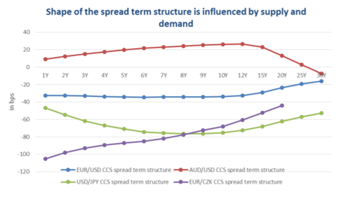
AUD/USD rises to a peak of ~20 at around 10-12-years but then falls to ~-5 at 30-years. EUR/USD is flat to 12-years but then rises to 30-years while USD/JPY falls to 8-years and then rise to 30-years.

Why do they have different shapes? This is primarily driven by supply and demand at different tenors.

Shorter tenors, say less than 2-years are generally dominated by liquidity requirements. These can change quickly, and these tenors can see quite a bit of volatility as supply or demand for one or both currencies drives the market spread. For example, in the GFC, demand for USD was intense which caused currencies like EUR to move to very negative spreads as market participants borrowed the USD and lent the EUR to fund their USD requirements through FX Forwards and cross-currency swaps.

The middle tenors, say 2 – 10 years are often dominated by medium-term debt issuance. Currencies where the domestic firms issue offshore and swap the proceeds back to their home currency (like AUD) will have demand to borrow the domestic currency via the cross-currency swap. This typically results in an upward-sloping curve in these tenors. The opposite is true for currencies such as JPY where the investors are buying offshore assets and creating the onshore asset via the cross-currency swap.

Tenors greater than 10-years are often influenced by structured, long-dated products and their market demand. For example, at the time of the chart above, a number of very long-dated AUD/JPY FX options were embedded in structured products and then hedged in the cross-currency markets. This led to lower 30-year spreads in AUD/USD and higher spreads in USD/JPY cross currency markets as the demand was all from a single direction, driven by yield-starved savers within Japan.

Supply and demand vary considerably across currencies and tenors and will also change over time.

Why do some currencies have positive spreads while others are negative?

Much like the tenor arguments above, this is primarily a supply and demand issue.

Countries with structural requirements to borrow offshore will typically have positive spreads. The buyside, such as firms who issue the offshore debt, will receive the USD and pay the local currency such as AUD. This drives the spreads positive and consistent mid-tenor demand will tend to keep them positive.

Countries with more demand to invest in offshore assets will tend to hedge these in cross-currency swaps by paying the offshore currency and receiving the domestic currency. Japan is a very good example of this tendency, and we can readily see this as negative spreads in the cross-currency swaps as they lend into the JPY leg of the swap pushing spreads negative across most tenors.

Calculating spread margins for buy-side clients

When hedging assets or liabilities, many buy-side firms will try to exactly match the cashflows on their offshore currency. For example, an issuer of a USD fixed rate 5-year MTN would prefer to match the fixed coupons and express the spread in their own, domestic currency.

The following example is for AUD/USD (where this is common).

The buy-side firm:

1)      Issues USD debt fixed rate

2)      Enters cross-currency swap where:

a.       Issuer receives USD fixed rate to align and offset debt coupons.

b.       Issuer pays AUD floating rate plus margin M1.

The sell-side counterparty will look at it like this:

1)      Pay USD fixed rate/ receive AUD floating rate plus margin M1 with Issuer.

2)      Price and hedge by:

a.       Receive USD fixed rate/pay USD floating rate plus margin M2 (based on the fixed rate of the issue and the prevailing market rate).

b.       Receive USD SOFR plus margin M2/pay AUD floating rate plus margin M1

The sell-side counterparty will calculate M1 based on the market rates current at that time.

Convexity

When calculating M1, the sell-side counterparty must use M2 from the USD single currency swap and the prevailing AUD/USD cross-currency spreads, USD SOFR/ AUD + M3.

We have an equation which looks like this:

1)      AUD/USD market: USD flat/ AUD + M3.

2)      Add M2 to the USD side: USD + M2/AUD + M1.

3)      Solve for M1.

4)      Note that unhelpfully, M1 ≠ M2 + M3 because of ‘convexity’.

The convexity arises because the discounting rates in AUD and USD are different so the present value (PV) of 1 basis point in USD ≠ PV of 1 basis point in AUD. When converting spread points on one currency to the equivalent in another currency, this difference must be accounted for.

When the spreads are large (say 100 basis points) and/or the discount rates are very different (e.g., AUD and JPY) then the solution for M1 in point 3 may be very different to the simplistic approach in point 4.

This problem is very real in crosses such as AUD/JPY. Both refer to the USD curve, but the cross will have a margin on both the AUD and JPY legs of the swap when combined. This needs to be resolved correctly in the pricing and convexity can be a confusing factor in the final rate.

XVAs

My last point in this blog is about the XVAs.

Many buy-side participants may not collateralise their derivatives and are therefore subject to CVA and FVA (and perhaps other XVAs) adjustments to the cross-currency pricing. These adjustments can be very large and sometimes dominate the spread shown to the buyer without these adjustments. FVA in particular can be very positive or negative depending on the currency pair and the direction of the trade.

Since XVAs can be so significant, buy-side firms should be vigilant on their pricing and implications to the outcomes.

Summary

The pricing of cross-currency swaps is often a complex and opaque process for many firms.

• Currency pairs and crosses have different spreads across tenors and often different term spread profile

• Some have positive and some have negative spreads

• Convexity will be important when dealing with larger spreads used to properly hedge exposures such as debt issues.

• XVAs can be a significant input to the pricing.

Martialis has significant expertise in pricing derivatives including cross-currency swaps.

We also work closely with Tokenhouse which is a new company established to address the buy-side challenges of structuring and pricing derivatives and wider treasury products. We will bring more news on this later.

Cross-currency swaps are a very useful product for many firms both buy and sell-side. Understanding the dynamics of pricing and the impact on the final trade is essential to getting a fair and appropriate outcome.

The decision to do nothing is still a decision…

My latest blog introduces a long-held area of personal interest and an emerging area of activity for our firm: that of assisting market-exposed clients establish frameworks that lead to more bankable performance compared with alternatives (including doing nothing).

In making the introduction I’m going to take the risk of leaning on the super-dry topic of decision-making under uncertainty in an attempt to explain how robust frameworks can promote higher-quality outcomes.

Along the way I’m going to unpack and focus on the question of hedging and the decision to ‘hedge’ (literally anything) in an effort to reinforce some key points.

Frameworks matter

Have you ever apprehended the arm-rest of a perfectly healthy airline seat while pretending not to be nervous in strong turbulence at 45,000 ft?

Let’s be honest: there’s no fun in being pitched around the ceiling, and you probably weren’t alone in choking that arm-rest. Some of your fellow passengers are likely to have suppressed an urge to scream; others are likely to have considered some futile assault on the cockpit door.

Don’t believe me? Try Googling ‘crazy reactions to strong turbulence.’

Aside from the fact that modern cockpits have sophisticated locking mechanisms, the good news is that your decision to do absolutely nothing turned out to be the best decision you could make.

Why?

Because decision-making frameworks with flight-controls and safety-protocols honed in various fields of science, backed by a hundred-plus years of controlled-flight data, were set by experts long before you bought your ticket. The risk of a modern jet-liner crashing from turbulence, even the heaviest most randomly experienced, is today so small it doesn’t register in International Civil Aviation Organization data.

Arm-rests aside, the modern air traveller has no need for turbulence-hedges.

Frameworks matter in finance (a lot)

 Before I try and connect the quirks of aviation to the world of financial markets, ask yourself: would frameworks and protocols matter if instead of being crowded into an A-380 you were a passenger in a single-engine Cirrus SF50 Vision?

The answer is: they still matter. Size doesn’t make much difference when you’re dealing with gravity at 45,00 ft.

While the flight and safety protocols of the Cirrus may be different, the key point is that a framework is still crucial, perhaps even more so considering the 1,610kg SF50 has only one engine and no co-pilot.

Which brings me back to financial markets and the need for parties to be able to negotiate market turbulence: can the kind of lessons learned in distant fields like flight and engineering be turned profitably to use in financial markets?

My answer is a question: why not?

Operations Research has led us

Operations Research is the branch of knowledge that deals with methods to improve decision-making with an emphasis on advanced analytical methods. Why it is not so well known in financial circles is something of a mystery, but it is one of the key disciplines that have helped important fields make the world a better, typically safer place.

Consider this: the collected benefit of OR, from its earliest practical application in the desperate months of wartime Britain, to its influence on modern decision-making in healthcare, is hardly appreciated when it is even known to people in finance. Yet, like the opening-up of mass air-travel and the winning of wars, the potential value of better decision making in finance should not be underestimated. 

While OR is not instantly recognisable it can be applied to almost any field (and typically already has), and some apply it without realising it, others are applying it haphazardly.

We are starting to simply apply it to add value.

Hedging as one example

My interest in financial markets was sparked by the realisation that portfolio management involved decision-making under uncertainty. The more important the decision, the greater the uncertainty; the more I liked it.

At various times my roles involved the tricky decision of whether to hedge certain elements of businesses that I ran or was involved in. This led me to think about how to apply OR and other tools to aid my decision making, I found that without a robust framework I was lost at sea, or to resubmit the aviation theme; I was mostly bouncing around in market turbulence without a parachute.

Imagine you’re an investment-manager running a partially-international investment portfolio, and let’s say the USD exposure of your portfolio averages 33% through time (which is a bit low compared to a recent well-regarded National Australia Bank survey).

Market-savvy, you’re likely to know a bunch of things already:

1.       The 30-year annual calendar-year Hi-Lo range of the AUD/USD exchange rate is conservatively around 18% p.a., let’s stick with that,

2.       Higher than average ranges occur approximately once every three years, and these average 31.1% (annual ranges) when they do occur.  

Seated in the investment-manager role (it could just as easily be an import or export treasury role) you could infer some simple expectations based on the original market-neutral framework of Black-Scholes (ignoring logs, things are as likely to go up as down):

·       Your USD-linked portfolio is impacted by higher-range years on average once every three years

·       Average calendar years can be expected to result in moves of around 9% up or down

·       High-range years can be expected to produce moves of 15.6% up or down

All of which is unremarkable; but consider these points from back-of-the-envelope calcs:

·       At some point in your average year the USD-linked portfolio can reasonably be expected to either drag or enhance portfolio returns in the order of +/- 2.97%

·       In a high-range year the drag or enhancement can be expected in the order of +/- 5.13%

The point to be made here is that the decision to hedge or not hedge exposure is consequential.

A separate but related point is that for those exposed to the Federal Government’s YFYS framework (Your Future Your Super) the hedging decision may be of heightened interest given that it takes YFYS managers further into a relative-performance arena.

That is: consequential decisions, whether well-formed or pot-luck, will be open to heightened scrutiny in a competitive sector that rarely produces net returns above 9% p.a. (7-year net p.a.). 

So, what’s your framework?

Our experience has informed our approach, and that is to start by asking our clients some really simple questions, allowing them to self-test their current approach even if they never engage us:

1.       Does uncertainty drive consequential outcomes?

2.       If consequential, do you seek gain or protection from the exposure?

3.       Do you have an existing framework to achieve what you seek?

And so forth….

What we all too occasionally find is that even where well-considered frameworks have been established the currency hedging-decision is often unloved, and often taken as a separate decision rather than a high-quality element of a high-quality investment management process.

To mention a few of the challenges we see firms not addressing well are:

·       Some firms evidence framework-rigidity, others exceptional latitude (are we running a hedge fund?)

·       Robust approaches to determining currency cheap/dear are often strewn across multiple spreadsheets owned by multiple decision-makers – i.e., the antithesis of a framework

·       Tailored hedging product-suitability frameworks are often missing completely (premium illusion is real)

·       Tests for correlation (natural hedges), regular or otherwise, are typically missing

·       Stakeholder awareness is a problem (why did markets all rally 7% but we only made 3%?)

The last word

To leave you with a key message I’m going to turn to the words a professor of business history at Harvard Business School and Johns Hopkins University, Alfred D. Chandler Jr., who wrote that “unless structure follows strategy, inefficiency results”.

Mr Chandler’s theory is easy to quote, but what of the evidence it can work in investment management? As the Wall Street Journal recently found, Chandler’s approach has been found alive and well at a little-known US closed-end fund, Central Securities Corp, run by an even less well known manager: Wilmot H. Kidd III.

Wilmot H. Kidd III has racked up one of the greatest long-term track records in the history of investing.

Over the past 20 years, Mr. Kidd’s Central Securities Corp., a closed-end fund, has outperformed Warren Buffett’s Berkshire Hathaway Inc. Over the past 25, 30, 40 and even nearly 50 years under Mr. Kidd, Central Securities has resoundingly beaten the S&P 500.

Using Compounded Rates – A comparison of different methodologies in high volatility

My previous blog looked at the ways to use SOFR to calculate a term rate. Because SOFR is an overnight rate, users are obliged to transform this into a term rate such as 1-month to align with the settlement frequencies on financial products. This is typically done by averaging or compounding SOFR over the relevant period.

This blog looks at the impact of different methodologies during the periods of high SOFR volatility in 2008, 2019 and 2020. These dates were selected because they have large moves in SOFR over a short time frame resulting in significantly different outcomes for the compounded term rate. While this may be a relatively rare event, should we enter a period of increasing US overnight rates (Fed Funds) then this will be reflected in SOFR. Even minor differences in the methodology can lead to significant differences in outcomes.

Of course, you can set the SOFR rate upfront in the same way as LIBOR. This is Term SOFR and is available for licensing from CME. I will look at developments in Term SOFR in following blogs.

The term SOFR (small t) here is set in arrears once the final SOFR input is known.

A recap on the methodologies

I used this table in the previous blog to describe the basic methodologies used in creating a term SOFR.

In the previous blog I showed Lookback and Observation Period shift are quite similar in outcome for each hi.

In this blog I look at the Payment Delay and Lookback options only to show their relative performance in different conditions and for different lookback days.

2008 – the GFC effect

SOFR was not published until 2018 but the NY Fed has kindly provided a set of proxy SOFR rates derived from market inputs from much earlier dates including 2008. While this is not actually SOFR, it appears to be a good representation of the repo rates (SOFR proxy) from 1 August 2008 to 31 December 2008.

The following chart shows the rates over that period followed by 2 tables with the results for 17 September and 19 September 2008. I selected these 2 dates to demonstrate how a few days difference in the number of days for the lookback can give very different outcomes for the 1 and 3-month term rates.

SOFR was quite flat around 2.00% until 11 September 2008 (LHS red circle) when it spiked on 12 September and fell to 0.25% on 17 September. It then bounced to 1.82% on 19 September (RHS red circle) before continuing a volatile fall to near zero by 31 December 2008.

The grey shading for the 5-day lookback demonstrates how volatility can impact the outcomes for the methodologies.

Both the 1 and 3-month term SOFR rates differ because the input rates to the calculation are very volatile, and the difference of a few days can include or exclude outliers in the data set.

2019 – the SOFR spike in September

SOFR was setting at around 2% for most of September 2019 but spiked to 5.25% on 17 September on technical liquidity issues. While this was unusual it still had an impact on the outcomes for term SOFR rates which did or did not include the spike. The chart and table are below.

The payment delay does not include the spike but the lookbacks both have this feature in the data sets. This results in a 17-19 basis point increases in the 1-month term SOFR and 8-9 basis point increases in the 3 -month term SOFR.

Again, we see the impact of the choice of methodology on the outcomes for the term SOFR.

2020 – the COVID-19 impact in March

This period was quite volatile and presented 3 rapid falls in SOFR from 1.6% before 2 March 2020 to 0.00% by 18 March 2020. The red circle outlines the largest of these falls in SOFR between 13 and 16 March where SOFR moved from 1.20% to 0.26% over the weekend. The impacts are captured in the chart and table below.

Yet again, the methodology does matter. The 1-month difference between the payment lag (o days) and the 5-day lookback is almost 25 basis points! The 2 and 5-day lookbacks both include SOFR rates at 1.6% while the payment delay does not use that data. The outcomes are as expected with the lookbacks showing higher term SOFR rates than the payment delay.

Does this matter?

Last time we saw that the choice of methodology was not important when SOFR is not volatile: this has been the case in the recent past.

But the methodology does matter in periods when SOFR is volatile (2008), subject to a liquidity event (2019) or has a sudden change based on Fed activity (2020).

In these cases, we can see that the use of a 0, 2 or 5-day lookback can have very significant impacts on the term SOFR rate applied to a contract or trade.

Read the fine print carefully and align your hedges

Although the actual methodology does not significantly impact the term SOFR rate when markets are calm and the Fed is not moving the target band, this is not always the case. We have seen in this blog that a simple change of the lookback days can lead to important and meaningful differences in the final term SOFR.

So, as we stated in the previous blog, read the contractual terms very carefully, it does matter! And make sure you align the hedges as well.

Do you really want the risk of a mismatch in the timing of the SOFR data used for the calculation of the term SOFR? As we have seen, this can matter a great deal and can be eliminated by correct alignment of the hedge to the risk.

The next blog will look more at CME Term SOFR and how it performs relative to the compounded term SOFR.

Data may not lie, but it sure can conceal…

In our Insights blog from September, we explored the value of independence when considering a review of dealing desk performance, leveraging the events surrounding a well-known historical incident to make some hopefully valuable points. In this post I follow-up on the topic by sharing some insights into how a simplistic acceptance of a firm’s existing performance and/or risk data, justifiably derided as the ‘tick-and-flick approach’, can lead to downstream problems.

Spot the elephant

Lee Baker

Lee Baker is an accomplished data scientist, software creator, CEO of ChiSquared Innovations, and author of at least fourteen books on how to work with data. His almost perfectly-named firm has a vision to “produce statistical analysis systems that take you ‘from data to story’ with as little fuss as possible.”

I was drawn to Lee’s earliest work in 2017 when his hit, Truth, Lies & Statistics: How to Lie with Statistics seemed to confirm a former boss’s suspicion that when Powerpoint was used in business the content was nine-tenths deception. But Baker’s clever rearrangement of a quote often attributed to Mark Twain was also catchy; though Twain borrowed from Benjamin Disraeli who is reputed to have remarked that: “There are three kinds of lies: lies, damned lies, and statistics.”

Truth, Lies & Statistics is an easy and fun read, and with chapters like “Pirates Caused Global Warming” (debunking the Post Hoc fallacy) it’s like a crib book for the statistically devious. But while Twain and Disraeli risked painting actual statisticians in a bad light, Baker mounts a partly-convincing defence, turning his sights on those who might use statistical tricks to “hoodwink and otherwise dupe the unwary.”

What Baker’s works reveal is that there are lots of ways data can be manipulated or misrepresented for gain or deception. 

The data challenge

In modern finance the average firm produces quite staggering amounts of data, and there are many ways it is ‘manipulated’ for good or not-so-good, but with the rather obvious rider that it is overwhelmingly intended to be for good. For those faced with the daily consumption of Fantasia-inspired bucketloads of information it can be useful to ask if you truly understand what the information is telling you? But we also suggest you ask: what is it not telling you?

At Martialis, our view is that practically none of the data ‘manipulations’ used to create 1st and 2nd line reporting were ever devised to “dupe the unwary” as Lee Baker put it. In truth, they’re purpose-built, specifically designed to guide and inform, and firms spend millions trying to ensure this. Despite this, our experience has shown that even the most perfectly presented reporting, containing data of the highest quality (clean), can still dupe both the wary and the unwary, and this can create problems if left unchecked.

What has led us to this seemingly contentious conclusion?  

It would be easy to answer this by simply reminding readers that humans are fallible, but there are often deep-seated reasons why data can cause problems, which we broadly catalogue as:   

• Complacency, inertia and variability of experience;

• Misinterpretations, and/or misunderstandings;

• Misadventure, not exactly “the dog ate my report,” but variants that might surprise, including reporting-line and staffing changes, particularly of management;

• Information overload, a not uncommon problem in a heavily regulated industry; and

• Lack of reporting completeness and/or modernity.

And it’s this last category that I will expand on today: the lack of completeness and/or modernity in the 3rd-line space, drawing on recent work with clients and the directions we have been taking in our Dealing Desk Review practice.

Lessons from 2004

In my September blog-post I referred to a difficult moment in 2004-finance that shocked dealing desks across Australia and elsewhere (and upon which information can be readily found with any search-engine). What we know from the incident is that dealing staff sought and found ways to conceal unauthorised activity. We also know that senior dealing management’s interest in the underlying activities of the desk proved insufficient, and there were elements of complacency, misinterpretation of data, and some information-overload thrown in for good measure (regulators did eventually note some 800 individual limit breaches had been concealed; so, data was likely piling up somewhere).

However, and this is key; the reporting at the firm which suffered the eventual loss did not produce red-flags of sufficient magnitude at high-enough points on the management-hierarchy to back-up those brave risk management professionals who did alert management to a suspected desk-out-of-control problem.

At this point I will re-emphasise the point I made in my September blog: an independent review of the flags that were being raised in 2003 and ‘04 would likely have saved millions.

Bigger lessons still

Through relatively simple research, we found that since Y2k there have been at least 47 dealing-desk losses of greater than US$100m magnitude, including the Australian loss of our blog. What’s striking is that a clear majority of these were experienced by well-regarded and major global financials.

Of these:

• Total losses (of the 47) amounted to U$101.6B at mid-2021 values,.

• The largest amounted to U$11.4 billion (2008).

• A great many more (that we couldn’t research) comprised losses of less than US$100 million.

• Of losses (by the amount lost):

o   78.7% were generated by firms that had a Big-4 audit relationship;

o   39.3% were generated by a Systematically Important Bank; and

o   10.4% involved non-linear derivative products (somewhat surprisingly)

• Not all involved fraudulent dealing activity.

Which has, at least in part, encouraged us to expand on the client-driven demand for Martials approach to data-analysis completed in prior years in this specialist field. 

What can we deploy (now)

Having commenced desk reviews in 2019, we have steadily grown the areas of this interesting capability, with focus on three broad fields:

1.       Discovery – developing a proprietary base-line view of the desk on which the need for deeper review can be determined:

a.       Type of desk

b.       Unusual or atypical attributes – returns/risk/other

c.       Peculiarities versus norms/peers

2.       Desk Conformity, with/to:

a.       The implied or present regulatory environment

b.       Industry standards

c.       Market best-practice

d.       Policy

3.       Desk Alignment, with/to:

a.       Strategic intent, e.g., sources of revenue and/or risk, type of desk

b.       Adjacent businesses, as stand-alone or as a component with

c.       The degree of complementarity

Answering interesting questions

• Does the desk generate actual outcomes consistent with its mandate and stated strategy?

• Does the desk demonstrate sustainability from a range of Martialis proprietary standpoints?

• Are there elements of performance/risk/funding that warrant deeper review?

• In generating revenue, is the desk conforming with regulatory and industry standards and expectations?

• Does the activity entail supervisory corner-cutting, individual or entity overreliance, or elements of questionable activity?

In the process, we catalogue and flag areas where a desk may be adrift from industry best-practice standards and methods. Our focus is on the alignment to your strategy and how this compares with similar desks at other firms.

We look at the performance over a number of years and your assumptions of revenue sources against the actual revenue in the Discovery phase. Our experience suggests assumptions and performances are often poorly correlated and a detailed investigation can improve business performance.

Using Compounded Overnight Rates – a basic guide

As markets move towards overnight rates and away from LIBOR (and other IBORs) there are a variety of ways to transform theses rates into a simple interest rate that can be used for the relevant period, say 1-month. My previous blog on the alternatives for term rates in USD looked at how these could be used to replace LIBOR.

This blog addresses the ways in which the overnight rates can be turned into a rate which is applied for a period such as 1-month (or 3, 6 etc. months). and how these are accessed in the USD SOFR market example.

As many have noted previously, when you use overnight rates to calculate a ‘term’ rate (i.e. one for that period) the actual result is not known until the end of each relevant period. The final rate is not published until the day following the final rate fix and many firms need a number of days to arrange for calculation and payment resulting in a variety of methodologies to accommodate this ‘inconvenience’.

Note that the term rate is not a Term rate such as Term SOFR. A Term rate is set at the start of the period whereas the term rate is not known until the end of the period. The terminology is a little confusing but it is commonly used.

Some basic concepts

Using SOFR as an example, the basic compounding and averaging calculations for each period are:

Some common methods for allowing for payments to be arranged

As mentioned above, the final SOFR rate is not known until the day after it is set and many firms need a few days to arrange for payments. The more common variants are payment delays, lookbacks (observation shifts or ‘lag’) and observation period shifts (‘shift’).

Each variant is in current use and often one is favoured for a particular product.

The difference between the lookback and the observation period shift is important.

A lookback preserves the relevant period and simply uses the ri from a certain number of days prior. This can have the disadvantage that the ri intended for a particular number of days may not be applied to that number in the calculation. This is the main reason a 5-day lookback is often favoured because it has a better chance of alignment than a 2-day lookback.

The observation period shift avoids this problem by moving the whole calculation back a number of days thereby ensuring the ri continue to align with the correct days.

NY Fed SOFR, SOFR Averages and Index publication

The NY Fed publish the Daily SOFR and a number of other calculations each day at 0800 ET. These are excerpts of the screens.

The SOFR rate (0.05%) is per day in the first screen and the 30, 90 and 180-day averages plus the index is also provided.

The ‘Average’ is actually the simple interest rate calculated using the compounding methodology but is referred to as the average. This can be confusing but it is accepted by markets.

The index is the discount factor calculated each day using the SOFR rates and measures the cumulative value since 2 April 2018. The index can be used for the observation period shift methodology by finding the dates and using the formula below. Note the index cannot be used for a lookback because the dates are no longer aligned to the appropriate SOFR rates.

The following tables are snapshots of the NY Fed pages for SOFR and then the Averages and Index.

Does this matter?

The simple answer is ‘not at this time and with these rates’.

In this table I have used 8 decimal places to show there is little difference in the rates. Most product and contracts round to 5 decimal places so there would be no difference. But be aware that the NY Fed Averages are actually the compounded 90-day and do differ from the more commonly used 3-month period.

It is also worth noting that the compounded and averaged calculations of the rate are different.

Read the fine print

It is clearly important to know if the methodology is compounded or averaged because this will almost always lead to different rates. Both calculations are used in USD products.

Likewise, it is important to use the correct dates: 90-day or 3-month as this also matters to the final rate.

So, read the contractual terms very carefully, it does matter!

The next blog will look more into how the methodologies can impact the rates when rates are SOFR higher and/or have greater volatility. In these cases, the choice of lookback or observation period shift can matter.

Lessons on the road to cessation – the JPY capital markets

In our last post we resorted to a smorgasbord metaphor to help carry the point that in the post-LIBOR world market participants have so many alternate benchmarks they should carefully evaluate for choice. Given some of the feedback, we thought it worth following up with a close look at progress in Japan. It’s a jurisdiction with a massive savings pool where benchmark choices appear somewhat different to USD and GBP.

What we found was more than interesting.

The USD market – real progress since 2019

On July 31st 2019, the world’s first SOFR deal settled; JP Morgan was issuing another piece of its regular preferred stock offerings. As Risk.Net sagely noted at the time, the issue had a “first-of-its-kind provision buried in the small print.” What they were pointing to was that the floating leg would “pay a forward-looking term rate based on SOFR, the secured overnight financing rate.” The $2.25 billion deal was set to pay a fixed-coupon of 5% through to August 1, 2024 thereafter switching to “a floating rate of three-month term SOFR, plus a spread of 3.38%.”

Which was quite brave of JP Morgan; term-SOFR had not yet hurdled regulatory approval let alone seen the light of day, and there could have been no certainty regarding the future viability of Term-SOFR.

Today, USD issuance in a SOFR format is more common than LIBOR, so much so that the CME run a SOFR Issuance Tracker, offer a wide suite of futures, and OTC market-makers have followed the obvious trend. Market conventions appear to have largely settled.

Looking into issuance data, what we note is that the hallmarks of a successful USD product transition are falling into place. Likewise, UK markets have carried-off a similar transition to their SONIA-based future, with markets now almost entirely absent GBP-LIBOR dealings. Thus, the crucial USD and GBP-based capital and financial markets appear to have the necessary features that promote their proper functioning:

For the sake of building up a point of comparison from which to judge the ARR scene in Japan, we review USD issuance since mid-2019.

Which to us is an impressive backdrop.

The Yen market – limited progress

In our comparative look at Japanese markets, we asked a simple question; what’s been happening in the market for JPY alternate reference rates (ARRs)?

Here is what we found for the same period (Mid-2019 onwards):

The Bank of Japan’s Cross-Industry Committee on Japanese Yen Interest Rate Benchmarks was established in August, 2018, and in November 2019, Quick Corporation’s forward-looking TORF benchmark was announced as the rate “most supported by public consultations.” The availability of an OIS-based TORF (in production since April 26th 2021) offers market participants a Japanese Term-SONIA lookalike in most respects, and it should be operationally easier than compounded alternates.

And JPY issuers have a range of other choices they can tap:

• TIBOR, the Japanese Bankers Association administered rate, has been calculated and published as "Japanese Yen TIBOR" since November 1995 and is NOT scheduled to cease when JPY-LIBOR does.

• Compound or Simple Interest TONA, could be thought of as Japan’s version of SONIA (unsecured, unlike SOFR), the modern form of TONA was introduced in 2016 and is administered and published by the Bank of Japan.

Digging a little further, we found that the single instance of TONA use in issuance was actually deferred until September 2026, coming as it does in the form of a convertible security issued by Mitsubishi Corporation:

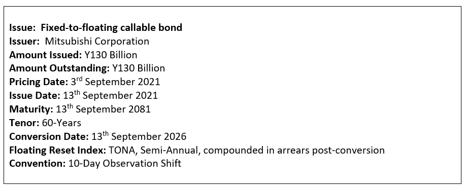
What this points to is that notwithstanding the Mitsubishi callable (which we note could be called before it ever converts), there is currently not a single floating issue referencing compound or simple TONA, and none referencing TORF whatsoever (further queries on this with major data providers confirmed that there have been no TORF security issues).

We will follow-up this analysis with a look at JPY-based corporate and syndicated facilities in coming posts.

Digging still further we took a deeper look at historic behaviour of the various choices, and noted that the annual volatility (a favourite measure, expressed in basis-points of underlying yield) of different ARR’s, including those where a particular convention might be used can be vastly different.

Consider the following distinctive range of volatilities over the past 10 years data:

JPY-LIBOR is clearly the most volatile, which is not unreasonable given LIBORs credit sensitivity, whereas TONA variants and TORF do not. But this opens the question of: why does TIBOR not travel at a similar volatility to JPY-LIBOR? And looking across time, why has TIBOR remained where it is despite the collapse in JPY-LIBOR and TONA to negative rates?

This suggests that those looking to Japan’s capital markets need to tread carefully around benchmark liquidity as well as expected benchmark performance, and those offering JPY drawings have to be able to find appropriate points of funding.

Are Japanese institutional features at play here?

To help us answer the question of why JPY markets have largely ignored the development of ARR’s we turned to macro-economic texts and some research on the features of Japanese finance.

These indicate that there are a range of features at play:

• Existing Bank of Japan interest rate settings continue to compress short-dated JPY yields, e.g., the JPY OIS Curve is negative to 4-Years, 9-Months

• Forward yield projections are partially implied by the extent to which the Bank of Japan is expected to hit its “Price Stability Target” of 2% at a time when Japanese Core Consumer Prices have been negative for all but one of the past twelve months

• The size of the household saving ratio in Japan (estimated at 11.4% percent for 2020) is the highest since 1994, adding to the existing Japanese savings pool

• To the extent that Japanese Corporations require funds there is a long-run preponderance of bank funding over bond funding

To gain a stronger feel for whether these features are right we turned to a Japanese based interest-rate dealer, Stuart Giles a Japan-based interest rate dealer

RB – Stuart, you’ve traded Japanese markets and rates for an extended period, can you give us a feel for why Japanese floating-rate issuance is exceptionally low?

SG – Traditionally there’s been an over reliance on bank funding vs domestic market issuance, but this has changed marginally in the Covid-19 era. Demand for floating-rate paper remains low as it provides yield starved local investors little in terms of carry or potential for capital gain. With essentially no prospect of higher floating rates here I don’t expect this to change. Floating-rate issuance also serves no practical purpose for hedging ALM mismatches

RB – Can you see the TORF benchmark developing momentum and liquidity in the manner of say Term-SONIA or SOFR?

SG – With the recent pickup in liquidity in TONA, this increases the robustness of the TORF benchmark given that TORF is based on the uncollateralized overnight call rate. There are still some important issues with the use of TORF to be addressed such as the establishment of the governance structure and an improvement of transparency in the calculation process however.

RB – If you had to guess, what would be the prominent Japanese benchmark in 10-20 years’ time from now?

SG – A further shift away from TIBOR may require additional pressure from regulators, so near term I’d expect it remains the dominant reference rate. The momentum is clear however that risk-free reference rates are the global norm, and Japan will likely keep moving in this direction also. TORF is well designed with advance fixing and thus predictability of cash flow like Tibor/Libor fixings. Once we have the availability of cleared TORF products I think this benchmark can become the dominant reference point for markets.  

Lessons

Our main take-away from these surprising JPY findings is that big assumptions can be quite dangerous. The Japanese economy and it’s institutional features and pressures have all ‘conspired’ to  ensure that Japan’s capital markets are different to GBP and USD, and other currencies, and thus the path to JPY-LIBOR’s cessation is quite distinctive.

For those considering tapping one of the world’s largest savings pools the lesson here is that it will pay to fully understand the range of factors that drive your outcome; which is likely to rest in the fundamental nature of the underlying benchmark.  

It really is a Smor Gås Bord…The decision on which post-LIBOR benchmark to use

In this blog we explore the increasing degrees of product-freedom available across post-LIBOR financial markets and the corporate finance suite. With the dizzying array of options seemingly available, we pose important questions for market participants to consider.

It’s not quite A Table Alphabeticall, and, somewhat amazingly, the Cambridge dictionary has only been available on-line since 1998, but they helpfully define the original Swedish noun ‘Smorgasbord’ as: a mixture of many different hot and cold dishes that are arranged so that you can serve yourself.  

Why on earth is this relevant in 2021 finance? Well, we’ve come to the conclusion that the Swede’s mix of smor (butter), gås (goose), and bord (table) is the near-perfect metaphor for the world of post-LIBOR finance.

We field a lot of finance questions from many different clients, and increasingly note that there is a wide and increasing array of ways to contract new deals. All of these have quite different ‘gives versus gets,’ and component pieces. Some are refined, some are quite raw and participants appear to have to figure out how to serve themselves.

And it may be difficult for bankers to accurately describe what’s on all those platters.

It’s now over four years since Andrew Bailey gave his momentous ‘The future of LIBOR’ speech. Despite the opportunity that many of us expected that LIBOR reform would bend market conventions toward conformity, the lived reform experience has been of the market response leading us to a world of far greater complexity.

Corporate finance and financial markets products are not going to click together with the simple LEGO-like efficiency of LIBOR products: new benchmarks are really quite different. Not just a little different; a lot different (think volatility).

So, what kind of basic questions should one consider when approaching the post-LIBOR deal ‘bord’?

• Do I really understand the underlying nature of the Alternative Reference Rate (ARR) I’m about to reference and use in contracts?

• How have ARR’s, or proxies, performed in terms of realised outcomes, annual ranges and historical volatility?

• What do ARR’s actually do at times of market disruption and heightened market volatility?

• Am I willing to accept the credit sensitivity of the financial sector remaining at play in my all-in cost outcome? The credit sensitivity is a feature of LIBOR and ARRs such as BSBY, Ameribor, CRITR and AXI.

• Could there be an all-in-rate advantage to accepting credit sensitivity?

• s the choice of ARR different for a borrower or investors?

Then, excuse fingers, there are real questions about what type of cutlery is available to help consume all these trimmings?

• Term RFR’s seem like a viable solution, but can I access them if regulators impose use-case limits?

• If I go term rate (credit sensitive or RFR) and need a derivative hedge, am I sure I can get one?

• If I get a hedge, will it work like traditional LIBOR hedges did in all cases?

• Speaking of that hedge, what about in three- or five-years’ time if use-case limits change and liquidity dries up?

• Cross currency swaps are two-day lagged, my cash instrument is five-day lookback, how am I (and my auditor) going to handle the exposure to basis risk and short-term liquidity?

• Can I get a convention match?

We’re not sure what part of the smorgasbord metaphor we can use for the other important considerations, but perhaps these are best described as condiments?

• My bankers insist on imposing an interest rate floor, isn’t that now at-the-money?

• Shouldn’t that floor also be embedded in the hedge?

• What’s this difference between period-floors and daily floors in the RFR facility, and why does it matter?

• Bloomberg Index Services Limited rates show some large differences in credit-adjustment-spreads between currencies and tenors in the ISDA fallback conventions, but my bankers want a one-size fits all margin in my multi-currency facility. What the gives here? 

To gain a better sense for the practical realities we spoke on this topic with Managing Associate, Yu Zhang, a specialist in the banking at corporate finance practice at leading legal firm, Allens Linklaters in Sydney.

“I think the smorgasbord analogy is quite apt.

The range of possible ARR/RFR conventions is somewhat daunting, then there’s the choice between credit-sensitive and essentially credit-risk free rates, and we think clients need to evaluate each of those areas very carefully. Then, for corporate finance and securities issuance, there are a range of risk-free-rate contractual facets that need to be considered, also carefully given the way these can influence economic outcomes.

Whereas a standard LIBOR corporate facility of old might contain three or four contractually meaningful elements (i.e., that can impact economic outcomes), when we deal with RFR-based deals, there are a lot more.

People should pick their meal from this smorgasbord carefully, and I think that view, that caution, is generally better understood than it was only a few months ago.” 

Yu Zhang, Allens Linklaters

What’s dawning on market participants is this: if you attempt major global cross-jurisdictional reforms and invite market regulators, the sell-side and the buy-side, and the loan-markets and derivative markets industry bodies to the same dinner party, not everyone wants a Big Mac.

Which is a recipe for confusion.  

For those charged with determining efficient capital costs or maximising returns we think it will be important to be able to cut through the confusion, and soon.

And lastly, try to avoid being the Gås!

Synthetic LIBOR - More devils in the detail?

Counterintuitively, the suite of LIBOR regulatory reform measures has often served to actually stoke market confusion. Judging from client reactions, the FCA’s latest consultation adds to the list of measures in the ‘confusing’ category. In this blog we explore the CP21/29 consultation, place it in its proper context, explain what may be causing the confusing, and work on demystifying it. All is not as it seems!

FCA CP21/29

On 29th September the UK’s FCA issued a number of important market notices, which included a seemingly innocuous consultation paper CP21/29, Proposed decisions on the use of LIBOR (Articles 23C and 21A BMR).

CP21/29 follows on from previous, related consultations:

§  CP 21/15 of May 2021, on the FCA use of critical benchmark powers, and

§  CP 21/19 of June 2021, on GBP and YEN LIBOR settings.

The key to understanding CP21/29 is that it pertains to two quite specific areas of benchmark reform, to use the FCA’s own language:

1.       The decision on whether and how the FCA might permit legacy use of GBP and YEN Synthetic LIBOR settings after January 1st, 2022.

2.       The question of whether and how the FCA might prohibit new use of overnight, 1m, 3m, 6m and 12m US dollar LIBOR settings after January 1st, 2022.

While we will explore the prohibition of use of US dollar LIBOR settings in a later post, we focus here on the linked questions around whether and how the FCA might permit legacy use of GBP and YEN Synthetic LIBOR settings?

Grounds for confusion?

Since the sweep of LIBOR reforms commenced major global regulators have uniformly urged market participants to deal with legacy LIBOR contracts in two broad ways:

1.       amending contractual fallbacks; or

2.       conducting active LIBOR-ARR transitions.

 For those contracts that might “prove unable to convert or be amended” regulators in major jurisdictions have focussed extensive past-year efforts trying to determine how best to a) define, and b) accommodate post-cessation treatment of “Tough Legacy” contracts.

Exemplifying this, the Bank of England established a Tough Legacy Taskforce within the Bank’s Working Group on Sterling Risk-Free Reference Rates while the UK Parliament passed laws in early 2021 giving the FCA wide powers to deal with this issue. Similar US legislation passed the New York State Assembly in April 2021.

The combination of these various efforts and widespread common use of the descriptor “tough legacy” has not unreasonably led market participants to develop LIBOR-cessation plans on the assumption that the sub-set of products deemed “tough-legacy” would likely be narrowly defined in any jurisdiction. Further, that reliance on a regulatory response for contracts other than those deemed “tough” would be unwise.

Consider the FCA’s language under section 3, The Article 23C legacy use power:

Our proposed decision

3.1 We propose to permit legacy use of these 6 synthetic LIBOR settings in all contracts except cleared derivatives (whether directly or indirectly cleared).

3.2 We do not propose to apply any limitations or conditionality to the above permissions, at least before the end of 2022.

While the CP21/29 is not a foregone conclusion (consult responses are requested by 20th October), LIBOR exposed parties could infer that it hints at a 180-degree turn on the part of the regulator, and we wouldn’t blame them: 

§  Far from being narrowly defined, the availability of a Synthetic LIBOR for legacy GBP and YEN contracts will be exceptionally broad.

§  Parties to non-ISDA LIBOR-referencing contracts that have not yet transitioned (in any way) can now consider a third option: doing nothing.

§  Parties that elected to repaper contracts, particularly via common switch provisions, or who have actively transitioned deals already, may feel they were somewhat misled in the lead-in to their decision-making.

These reactions are not unreasonable, but that is not to concede that they’re warranted.

Martialis View

The “proposed decision” outlined in Point 3. CP21/29, should not be read in isolation.

Significant practical constraints to reliance on Synthetic LIBOR remain and market participants should carefully evaluate whether to utilise it, particularly where more robust alternative paths are clearly available.

Synthetic LIBOR could be thought of as a makeshift substitute to robust fallback or active transition, but important considerations, not limited to the following, should be carefully taken into account:

1.       The FCA’s preparedness for an all-contract use case is not open ended

While they have the power to compel IBA publication of a Synthetic LIBOR for up to 10 years, the extent of a commitment outlined in CP21/29 is to end-2022, to wit: they do not propose to apply any limitations or conditionality to the above permissions, at least before the end of 2022.

To be specific, under ARTICLE 21(3) BENCHMARKS REGULATION – NOTICE OF FIRST DECISION, of September 29th, the FCA state that: the compulsion period shall be for 12 months starting immediately after the final publication of the 6 LIBOR Versions (GBP and YEN) on 31 December 2021 and before the 6 LIBOR Versions would otherwise cease.

The FCA will regularly assess Synthetic LIBOR (annually is likely) and may discontinue its publication prior to the 10-year maximum allowed.

This should give significant pause for consideration to those who might otherwise accept what presents as an easier path past the end-2021 cessation event.

1.       Term-RFR use case limits across derivative markets remain unsettled

While a jurisdictional divide on this question appears to have opened up between the UK and US (and Japan), it’s clear that UK regulators have misgivings over unlimited Term-SONIA use.

For those who may subsequently seek term-rate hedges to replace Synthetic LIBOR in legacy deals, a downstream lack of use-case availability or liquidity should be a consideration.

However, we do note the use of Term SOFR in large syndicated deals in the US is becoming more common.

2.       Parties with fixed-rate products

In examples such as the hedged-facilities common across asset and infrastructure-finance, active reliance on Synthetic LIBOR for both facility and hedge (provided it is uncleared) should be carefully considered.

Subject to points 1 and 2 (above) this approach may hold advantages where parties attempt to preserve existing fixed rates, a topic we are particularly familiar with.

3.       New products and reference rates

With what appears like a ‘stay on execution’ of GBP and YEN LIBOR the markets will have additional time to develop new products and alternatives which may include term rates. These may be more suitable for some participants.

Firms will need to remain alert to these developments as many end-users have shown a preference for term rates such as Term SOFR and BSBY.

Conclusion

For those who feel they could have avoided transition or repapering costs/disruption, a degree of frustration at the FCA’s poorly telegraphed announcement could be expected. We believe it will be important for participants to better understand this topic, and how it actually adds to choices that need to, like so much in the post-LIBOR finance, be carefully evaluated.