
Execution Costs – Mysterious or manageable?

One of the less well understood areas of finance is the impact of transaction costs on standard risk-reward models. While market makers with deep experience know that transaction size impacts costs, this is often not communicated to end market users in a transparent or quantitative manner.
In this first of a series of pieces, I use the efficient-market hypothesis to examine a number of hedging approaches and their impact on deal outcomes. I will show that averaging can be relatively efficient regardless of transaction size, but also that averaging’s benefits are positively correlated to deal size.
Crucially I use historic data to demonstrate that all-in cost probabilities can be quantified.
The Black-Scholes option pricing model transformed modern finance. Whereas prior to 1973 option prices could only be guesstimated, Black-Scholes presented a ground-breaking framework that birthed standardised pricing.
Coupled with the advent of the personal computer, Black-Scholes changed the manner and speed with which markets calculated risk. While arguments as to the limits of the model abound, elements of the original framework can be readily applied to advance our thinking in other domains.
In this piece I draw on the hotly contested efficient market hypothesis, which posits that market movements are essentially unpredictable, and might be thought of as a 50:50 hypothesis. I have often thought of it as simply that “markets are just as likely to go up, as they are to go down.”
As we shall see, while the hypothesis doesn’t perfectly hold, we can leverage it to assess the efficacy of different dealing execution strategies probabilistically. In this piece I use it to demonstrate that a carefully formulated execution strategy can minimise execution costs.
A market example
Let’s start by defining a simple scenario with key assumptions, of which I have chosen four:
As a hedger we are concerned about adverse market movements in the standard 3-year Australian dollar interest rate swap (IRS) market.
We are worried about adverse movements over the coming 3 months.
We have only two choices of how to execute our hedge:
a. At-Close Risk Cover - a single transaction executed at the end of three months, or
b. Progressive Risk Cover - transacting equal portions daily, accumulating in the outright exposure at the end of three months (i.e., approximately 1/60th hedged per day without exception).
All dealings are conducted at closing rates without execution costs.
I purposely chose the divergent forms of execution since they sit at extreme ends of the hedging spectrum. This is to highlight the importance of hedging strategy and the impact that deal size has on transaction costs.
For the sake of scenario framing, the following chart displays 3-year close-on-close swap yields from February 1991 until May 2023, which has been used in this analysis.

What becomes immediately obvious is that there has been a serial decline in yields (a generally rallying bond market) since 1991. We should remind ourselves that while historic outcomes don’t predict the future, the historic hedging outcomes show serial bias, and this has tended to favour swap payers.
Payers were favoured under At-Close Risk Cover ...
Under At-Close Risk Cover, the hedger is exposed to open market risk through the 3-month period, from initiation to close, with final cover being achieved only at the end-of-period closing price.
If the efficient market hypothesis held, we should expect a broadly 50:50 dispersion of favourable versus adverse outcomes, between payers and receivers.
However, as predicted, the long-term decline in 3-year yields within the dataset skews the outcome in favour of paying hedgers under the At-Close Risk Cover since 1991:
Payers, 53.46%
Receivers, 46.3%
Sum of favourable outcomes, 99.80%
Notice here that I have calculated the sum of favourable outcomes, which seems unnecessary. While this may seem superfluous the sum can be used to illustrate an important point and it gives us our results at base-100 which assists make our key point.
Notice, also, that in the case of At-Close-Cover the results do not precisely sum to 100%. This is because of 8,355 observations; a zero return was found on 17 occasions. On those dates neither payers or receivers obtained an advantage.
…. and Payers were likewise favoured under Progressive Risk Cover.
Under a Progressive Risk Cover model, it is assumed that it is possible to hedge the 3-month/3-year IRS risk at the mid-market daily close in equal daily proportions. This results in an ‘achieved transaction rate’ that is equal to the arithmetic mean of closing rates for sixty trading sessions.
The range of achieved rate outcomes (average rate minus initial rate) should still adhere to the efficient market hypothesis, that is: approximately 50:50 outcome split between payers and receivers.
Again, while our analysis uncovers a favourable bias for payers, it remains fairly close:
Payers 53.96%
Receivers 46.04%
Sum of favourable outcomes, 100.00%
And in this case the sum of favourable outcomes sums neatly to 100%.
What happens when we incorporate execution costs?
The two execution scenarios I have described here rely on the ability of hedgers to transact with perfect efficiency. That is: we’ve assumed hedging can be conducted at market-mid, which is obviously unrealistic.
So, what do we find in more realistic settings?
When transaction costs are included in our analysis, we find three things:
Favourable hedging outcomes are inversely related to transaction size under all execution approaches.
Progressive Risk Cover is more efficient than At-Close Risk Cover regardless of size,
The costs related to At-Close Risk Cover are positively correlated with increased transaction size, both nominally and relative to Progressive Risk Cover.
These findings will be unsurprising to market makers and those with deep markets experience. In fact, those who understand the nature of such costs will be right to ask, so what?
While we have proven the seemingly obvious, the point is:
The magnitude of transaction costs and their impact in large transactions, often fail to be quantitively defined for end users.
And yet there are few reasons for this lack of transparency.
While our experience in this domain would allow us to make reasonable transaction cost estimates, we have conducted soundings with market peers to arrive at indicative spreads.
The following graph collates these estimates of transaction costs and plots the impact they play on efficiency relative (based on 100 being perfectly efficient) to transaction size.

What does this show?
The difference in percentage-favourable results is quite stark.
· The blue line plots the percentage-favourable outcomes under Progressive Risk Cover,
· The red line plots the percentage under At-Close Risk Cover.
What we find is that under all deal size scenarios Progressive Risk Cover outperforms At-Close Risk Cover in terms of transaction costs. And as we noted, deal efficiencies decline as deal size grows for both approaches but maintains near-100 efficiency for Progressive.
Motive Asymmetry?
The field of behavioural finance is strewn with examples of the skewed perspectives found between those who seek to avoid risk and those who actively seek risk for profit. What should be clear is that regardless of motive, transaction costs can alter the standard efficiency paradigm no matter whether you are risk seeking or risk avoiding.
What should also be clear is that how you execute matters, and that the extent of that impact is magnified as deal size grows.
This makes specialist approaches to large or highly complex transactions a must, since a carefully formulated execution strategy can minimise both market risk and execution costs.
What next?
My next blog will focus on the risks associated with different execution approaches, again using progressive versus at-close scenarios and historic data quantitatively. This we will tie in with our work on premium illusion to demonstrate that there really is no such thing as a ‘free lunch’ when it comes to managing risk.
For those who would like to discuss the scenario, its outcomes, and/or the frameworks we use to quantify hedge-efficient approaches, please reach out at: info@martialis.com.au.
Term SOFR or not Term SOFR
My last paper made the case for the wider use of Term SOFR. My argument was based on the fact that the potential users of Term SOFR would only occupy approximately 1% of USD derivative turnover and would, therefore, hardly represent a systemic risk. Wider Term SOFR use, together with robust fallbacks, could significantly ease the operational risk and pressures on the end-users, i.e., the counterparties paying spreads to dealers.
On 21 April 2023, ARRC published ‘Summary and Update of the ARRC’s Term SOFR Scope of Use Best Practice Recommendations’ which reiterated and described their approach to the use of Term SOFR. The ARRC continues to recommend the restrictions on the use of Term SOFR which are reflected in the CME license agreement (CME is the administrator of the most commonly referenced Term SOFR).
The current restrictions will most likely continue to support the basis between Term SOFR and compounded SOFR, specifically Term SOFR is around 3 basis points above compounded SOFR for term (say 5 year) derivatives. This is because the restrictions encourage a one-way derivatives market where users can only pay Term SOFR but are restricted from receiving Term SOFR.
This paper looks at some alternatives to Term SOFR which may help end-users achieve the outcomes of Term SOFR without referencing Term SOFR and potentially offending the CME license conditions.

Let’s start with an example
Clients often have had loans linked to LIBOR and fixed debt issues swapped to LIBOR. The combination of floating and fixed liabilities has been managed using derivatives to the desired mix of LIBOR and fixed rates.
As assets are added or changed, the derivative market was a convenient and efficient way to trade into the desired exposure for the asset/liability balance. But this is about to change as USD LIBOR is discontinued from 30 June 2023. From July 2023 the USD market transition will force market users to alternate reference rates, including compounded SOFR, Term SOFR among others.
In the current system, a loan referencing Term SOFR can be hedged to a fixed rate using a derivative, so in this situation there is essentially no change from the situation faced under LIBOR.
However, using a derivative to swap a fixed rate debt issue to Term SOFR is not encouraged (ARRC recommendations) or permitted (CME license).
This is very clear from Scenario 7 in the ARRC publication reproduced below.

This is a significant change from the LIBOR experience.
The end-user may have a preference for Term SOFR referencing liabilities which is allowed via a loan but cannot be achieved by swapping a fixed rate debt issue to the same Term SOFR. The only way forward is to swap the fixed rate to compounded SOFR and run the basis risk between Term SOFR and compounded SOFR.
This is hardly ideal and potentially introduces new interest rate and operational risk.
Can you manage this risk using a basis swap from SOFR to Term SOFR?
The ARRC recommendations appear to allow this activity. Specifically, Scenario 8 shows the following transaction:

The accompanying commentary seems to imply this activity is permitted but the two scenarios below would not be in the spirit of the ARRC recommendations:
swap fixed coupons to compounded SOFR; then
swap compounded SOFR to Term SOFR (Scenario 8).
This does not appear to be permitted in the CME license as the Term SOFR risk is not embedded in a cash instrument, i.e., a loan.
So, the following arrangement of an end-user issuing fixed debt, receiving fixed/pay compounded SOFR and simultaneously receiving compounded SOFR/pay Term SOFR in a basis swap would not, in all likelihood, be allowed or, at the very least not be encouraged.

So, we appear to be left in a difficult situation where the end users may be forced to manage Term SOFR and compounded SOFR where previously they were only exposed to LIBOR.
Other ways forward for end-users
Many clients do not wish to manage the Term SOFR/compounded SOFR risk which they would acquire as part of a loan and fixed rate debt liability combination.
However, all is not lost. This could be managed with an active approach to the coupon dates of the debt and the calculation dates of the derivative.
Approach 1 – manage compounded SOFR to Term SOFR for a fixed debt issue:
Trade with the dealer as receive fixed/pay compounded SOFR (permitted) with terms and dates matching the debt issue.
Each rollover (coupon date), pay the USD OIS (1, 3 or 6-month as appropriate) to swap the compounded SOFR to a fixed rate to replicate Term SOFR.
While this approach achieves the desired outcome of fixing the SOFR rate for 1, 3 or 6-months, there are some challenges:
The operational risk of diarising and executing the USD OIS trades needs to be closely managed.
Term SOFR is calculated from rates across the CME trading day (see note below) and there may be slippage between Term SOFR, and the USD OIS rate traded on the day.
It is important to carefully match the settlement dates for each leg to ensure there is minimal impact on the cash management which could attract significant costs.
This approach is actually quite effective and could be a practical alternative to Term SOFR under circumstances where Term SOFR cannot be referenced.
Approach 2 – choose a point in time for your firm to fix the rate
In this approach, the firm decides on a specific time to transact the USD OIS and accepts there will likely be a difference from Term SOFR.
This is operationally much easier but can provide tracking errors if other components of the portfolio are referencing Term SOFR.
Term SOFR calculations and timing
Term SOFR is calculated in a very different way to the current USD LIBOR.
USD LIBOR is determined at a point in time, specifically 11 am London. If a firm were trying to replicate LIBOR, then trading at 11 am London in a market closely connected to LIBOR (e.g., a single period swap) would likely have little slippage.
However, Term SOFR is not calculated at a point in time.
Term SOFR is calculated as follows (CME description):
‘A set of Volume Weighted Average Prices (VWAP) are calculated using transaction prices observed during several observation intervals throughout the trading day. These are then used in a projection model to determine CME Term SOFR Reference Rates. Full details of the calculation methodology are available on the Term SOFR webpages.’
If you wish to replicate Term SOFR, you will need to trade a proportion of the USD OIS risk at each time CME accesses the price for the VWAP. This is made even more difficult because CME uses random times in each time bucket!
In practice, CME uses fourteen , 30-minute intervals with random time sampling which is not possible to exactly replicate without knowing the timing of each sample.
In practice, this makes it difficult to manage a USD OIS process to replace Term SOFR
USD OIS trades to replicate Term SOFR
Our analysis of USD OIS and Term SOFR since May 2019 (when Term SOFR was first published) gives some comfort that a practical approach could be found.
Example 1 - Trade half the USD OIS risk CME near market open and the other half near the close.
Average slippage is 1 basis point (bp).
Standard deviation is 4 bps.
Maximum is 26 bps.
Minimum is -22 bps.
The average and standard deviation are quite acceptable to many firms, but the outliers (maximum and minimum) are less attractive outcomes as the slippage is substantial.
The average slippage is within 2 standard deviations for 99.9% of time which may provide some comfort.
Example 2 – Performance over a 3-year quarterly swap traded each day.
Over the twelve rate fixes in a 3-year quarterly swap, the statistics are:
Average slippage is 2 bps.
Standard deviation is 1 bps.
Maximum is 4 bps.
Minimum is -1 bp.
The averaging process appears to be quite effective, with the maximum and minimum much reduced.
Over a 3-year swap, there may be some significant slippage days but, on average, the total outcome may be acceptable.
Summary
The recent ARRC announcements include recommendations which may allow end-users to hedge a wider group of Term SOFR exposures. But CME licensing still appears to restrict the use of Term SOFR to cash instruments and derivatives directly linked to those cash instruments.
Should the CME position change, firms could reconsider the Term SOFR use case.
In the meantime, there are practical and effective ways to replicate Term SOFR, some of which are described above.
But there are some risks and caveats:
Term SOFR is difficult to match exactly using USD OIS trades because of the timing and random nature of the Term SOFR calculation.
There can be slippage between USD OIS and Term SOFR which may cause tracking issues if parts of the portfolio reference Term SOFR.
There are operational aspects of trading USD OIS which need to be closely managed including date and settlement timing.
On the positive side:
The slippage appears to average out over time and across the rolls for a multi-roll swap.
A process could be put in place to manage the USD OIS trading and achieve quite acceptable rate fix and operational exposure.
In summary, if you need Term SOFR but are not able to access it for licensing reasons, there are alternatives.
How can Martialis assist?
Martialis can assist in this process by:
Designing appropriate operational procedures to manage the USD OIS trading and risk management;
Providing practical advice on establishing trading relationships;
Transacting and recording the USD OIS trades to ensure date and settlement matching;
Calculating any slippage to Term SOFR; and
Monitoring risks and pricing requirements.
While replicating Term SOFR appears to be complex, our experience shows this can be managed effectively and methodically if processes are robust and established proactively.
The Case for Wider Use of Term SOFR

In my last paper I looked at the trends in USD derivative turnover from BIS Triennial Surveys 2010 – 2022. In this paper I focus on the 2022 Survey and how it supports the wider use of Term SOFR than is currently permitted under existing use limits.
Many of our clients have concerns that SOFR is difficult to use compared with LIBOR. Most of their issues are related to operational problems, forward cash management and accounting calculations. LIBOR, as a forward-looking rate allows clients the time to manage their processes before settlement, whereas SOFR is a daily update which causes additional effort and forecasting. Term SOFR appears to be an easier transition as it shares many of the more desirable attributes of LIBOR.
Simply put, Term SOFR presents an easier transition from LIBOR than is compounded SOFR: CME’s own data tends to support this.
In the past I have looked at the use case for Term SOFR. Risk.net has published on this topic a few times in 2021, 2022 and 2023 outlining the various rules which are currently restricting the use of Term SOFR.
While many people, including myself, support the ARRC and Fed view that widespread use of Term SOFR may be problematic, I also believe that some easing of the restrictions may benefit end-users and not present systemic risks. This is supported by the Survey results as I explain below.
This paper looks at the 2022 BIS Triennial Survey for a breakdown of the users of SOFR and LIBOR. We can reasonably assume the LIBOR users will become SOFR users after 30 June 2023 (i.e., LIBOR cessation) so we can look at the total as a reasonable approximation of market turnover and user mix for SOFR.
Also, we could assume SOFR turnover is at or probably greater than in 2022 based on the trend in USD turnover to higher turnover over the past 10 years.
Firstly, let’s look at the product breakdown per participant grouping.
Turnover of USD derivatives by market participant groups
The Survey does provide some breakdown of the turnover of USD per market participant type. The trades are reported by Reporting Dealers and they separate their trades with other counterparties as follows:
Reporting Dealers – other banks reporting turnover;
Other Financial Institutions – financial institutions which are not Reporting Dealers (e.g., investment funds); and
Non-Financial customers – End users not included in the 2 groups above (e.g., corporates).
There may be derivative transactions between firms who are not Reporting Dealers: these trades would not be included in the Survey. Such trades could be between Other Financial Institutions so their market share may be even larger than that in the Survey.
The following chart shows the breakdown and the market percentage of each group.

The main points I see here are:
Overnight Index Swaps (SOFR) and LIBOR derivatives have comparable turnover.
Other Financial Institutions are the dominant payers with 80% of the total (SOFR + LIBOR) turnover.
Trading between Reporting Dealers is19% of market turnover and considerably less than the trading between Reporting Dealers and Other Financial Institutions.
Trading with Non-Financial customers is a minor part of market turnover and only represents 1% of the market.
Where is the turnover located?
USD is the largest derivative currency by turnover in the Survey as shown in the following chart.

Focusing on the USD, the turnover per country is varied as shown in the next chart.

USD derivatives are predominately traded in USA and UK with some turnover in other countries as well.
Conclusions from the Survey
The 2022 Survey is very clear that:
USD derivative trading is the largest by currency (44%).
The majority of that trading is in USA (68%) followed by UK (24%).
Trading between Reporting Dealers and Other Financial Institutions dominated the trading (80%).
Trading between Reporting Dealers and Non-Financial customers is a very minor component (1%).
As the USD derivatives markets, and presumably debt markets, move from LIBOR to SOFR, I reasonably expect the four points above to continue to be relevant.
How does this impact the use of Term SOFR?
The ARRC and Fed have reiterated their view that the use of Term SOFR should be restricted to a narrow range of products as described by Risk. The CME license terms for referencing Term SOFR reflect the ARRC recommendations and effectively prohibit using derivatives except between dealers to customers to hedge Term SOFR debt to a fixed rate.
The reasons provided by ARRC include to restrict the use of Term SOFR include:
avoiding a repeat of LIBOR with Term SOFR;
inter-dealer trading of Term SOFR could grow rapidly if permitted; and
trading Term SOFR could cannibalise trading SOFR itself.
The main fear is that easing restrictions on Term SOFR to allow for more use by end-users could unleash a torrent of inter-dealer and dealer to customer trading.
The 2022 Survey results do not appear to support this if trading Term SOFR had some restrictions to support dealer-customer and limited dealer-dealer trading.
The trading with end users in LIBOR (no restrictions and the vast majority of this trading based on my last paper) and/or SOFR (minimal in 2022) is only 1% of total market turnover in USD derivatives.
If all the LIBOR trading for Non-Financial customers is replaced by Term SOFR then it still only represents 1% of the market.
If interbank trading of Term SOFR was allowed (under certain restrictions) then it may also be around 1% of the market to clear offsetting risks between dealers.
So, even with a relatively unrestricted approach to allowing Reporting Dealers to trade with Non-Financial customers, the percentage of market turnover could be expected to be in the 1% – 2% range which unlikely to create a systemic problem if Term SOFR is discontinued sometime in the future.
Summary
The BIS 2022 Triennial Survey has many interesting features.
Among these is the interesting fact that trading between Reporting Dealers and Non-Financial customers is approximately 1% of market turnover in USD derivatives.
This has important implications for the use case for Term SOFR.
If trading in USD derivatives referencing Term SOFR is restricted to Non-Financial customers, then it is likely to be similarly around 1% of USD derivative turnover if all LIBOR and SOFR trading references Term SOFR.
This is not significant and would be unlikely to present systemic issues if Term SOFR was discontinued at some time.
Of course, contracts referencing Term SOFR would have fallbacks to accommodate a permanent cessation of Term SOFR.
I believe there is a good argument to allow wider use of Term SOFR for end users. A moderate relaxation of the CME licensing rules would allow a more balanced market (i.e., Term SOFR to fixed and fixed to Term SOFR derivatives) and address the reasonable concerns of the end users in the transition from LIBOR.
Bidding credit sensitivity adieu…

Credit sensitive benchmarks have been fundamental to corporate finance for many years. The loss of this sensitivity adds a systemic burden to deposit taking institutions. Why? Because corporate loan books no longer adequately reflect and compensate for the funding risk in the manner of the LIBOR-based system.
The magnitude of this mispricing depends on the extent to which corporate assets pervade bank balance sheets and the adjustment that bankers have made to lending margins. With banking sector credit risk returning to prominence recently, it is timely to look at this annoying, obscure, yet potentially impactful problem.
Our analysis concludes that while US banking market capitalisation has notably rebounded from GFC lows and appears capable of withstanding a major credit induced event; post-Libor risk-free rates may not adequately reflect the risk undertaken by lenders. This potential interest forgone is of a material magnitude.
Hypothetical Interest Forgone under SOFA during the GFC
We described some important work done by Professor Urban Jermann in our post of August 2022.
Professor Urban is Safra Professor of International Finance and Capital Markets at the Wharton School of the University of Pennsylvania, and we showcased his major work from 2021:
Interest Received by Banks during the Financial Crisis: LIBOR vs Hypothetical SOFR Loans.
This estimated the amount of interest that would likely have been forgone by US banks had US business loans been indexed to SOFR during the GFC:
“The cumulative additional interest from LIBOR during the crisis is estimated to be between 1% to 2% of the notional amount of outstanding loans, depending on the tenor and type of SOFR rate used”.
With cumulative interest forgone estimated at:
U$32.1 billion if loans had instead followed compounded SOFR; or
U$25.0 billion had they followed Term SOFR
To recap, these numbers represent the hypothetical interest income foregone if corporate facilities had been indexed against the major SOFR variants over the period 1st July 2007 and 30th June 2009.
To contextualise the GFC moves, 3m LIBOR versus 3m SOFR Overnight Index Swap (OIS) rates are plotted on the following graph. This credit sensitivity proxy is generally known as the LOIS spread.

The LOIS spread averaged 10.7 basis points for the five years prior to July 2007. This average LOIS spread rose to 89.1 basis points through the GFC, as defined by Professor Jermann.
A non-trivial amount
In a follow-up article in Knowledge at Wharton, editor-writer Shankar Parameshwaran highlights what Professor Jermann was driving at:
“The $30 billion in interest income due to the credit sensitivity of LIBOR is not a trivial amount”.
Inviting hurried back-of-the-envelope calculations, Parameshwaran calculates that:
“On March 6th, 2009, when bank share prices tanked, the top 20 commercial banks from 2007 had a combined market capitalization of $204 billion.”
According to NYU-Stern School of Business, forward price-earnings ratios for money center banks today sit at around 9x earnings.
Those wanting to interpolate what might have been should take care to note that Professor Jermann’s calculations were for hypothetical interest foregone over two years, whereas P/E ratios are based on annualised earnings measures.
Nonetheless, sector annualised interest forgone of between $12 and $17 billion (i.e., halving Professor Urban’s numbers) in an environment where stocks are trading on 9x multiples is very worrying, especially considering the sector market cap of only $204 billion.
2023 – What of the situation today?
Taking Professor Urban’s raw calculations and assumptions and applying sector asset growth, US banks across 2023/24 would likely forgo:
U$59.4 billion if loans follow compounded SOFR; or
U$46.3 billion if loans follow Term SOFR
This is a simple estimate if the credit moves of the GFC period are replicated in the coming two-year period; but system risk appears much lower given the expansive sector market caps.
For the sake of comparison, the market capitalisation of the 20 largest financials in the US sits today at around U$1.54 trillion at mid-March 2023 by Martialis calculations (U$1,541.29 billion to be precise). This represents an impressive rebound and growth of 755% since the height of the GFC.
Corporate lending has grown far less quickly.
According to the St Louis FED, total financial assets of the domestic US financial sectors grew only 85% over the corresponding period (a surprisingly large lag). For the sake of framing, it’s worth noting that the US economy is only a third larger than March 2009 in terms of annualised real GDP, so we’re within reasonable ballpark.
This suggests that the system could handle GFC like conditions, but that the interest likely forgone if GFC-like conditions re-emerge, is still quite material.
What of the latest credit stress event?
To simplify how we look at credit stress we’re starting to favour Invesco/SOFR Academy USD Across-the-Curve Credit Spread Indexes, known more generally by their acronym ‘AXI.’
AXI is starting to gain interest given its constituent make-up and methodology, and we like the clean picture of credit sensitivity it provides in USD:
AXI is a weighted average of the credit spreads of unsecured US bank funding transactions with maturities ranging from overnight to five years, with weights that reflect both transaction volumes and issuances.
AXI can be added to Term SOFR (or other SOFR variants) to form a credit-sensitive interest rate benchmark for loans, derivatives, or other products.
The historic picture of AXI across 1m, 3m, and 6-month tenors from 2018 is as follows:

Credit sensitivity is highlighted over the period of COVID market stress and more recently as bank funding costs have risen with the Silicon Valley Bank and Credit Suisse events of early 2023.
For those interested in further AXI resources, please refer to:
How is AXI tracking the current stress?
Here I compare 3-month AXI with 3-month LOIS (LIBOR-OIS) over an analogue period, starting 90-days prior to the largest jump above one standard deviation in LOIS from 2007, which occurred on 9th August 2007.
While the base of AXI commences somewhat higher than LOIS, at +19.3 versus +8.8 basis points in the ninety days to Day-0 (identified by the dotted red line), the credit sensitivity of the subsequent period shows remarkable similarities at the start of both periods of credit deterioration.

Conclusions
What is clear is that despite the move to risk-free rates (RFRs), rational investors remain rational; demanding higher risk premiums to compensate for the risk of funding banks.
What’s less clear is the extent to which banks are able to pass-on a higher cost of funds to cover their various assets; and this is a systemic problem.
While higher rates are almost uniformly beneficial across mortgage and smaller variable finance segments, it’s not clear how banks compensate for the absence of LIBOR-like credit sensitivity in their corporate assets.
With these points in mind, we encourage bankers to ask three questions:
How long will banking sector credit remain elevated?
Are we receiving sufficient compensation for corporate lending in a risk-free-rate world?
Should corporate loan margins be recalibrated accordingly?
Widespread failure to address these seems to us to have rather obvious consequences.
The Triennial BIS Survey – USD Derivatives
Every three years I eagerly await the BIS Triennial Survey as it rarely fails to surprise. The 2022 Survey was announced in October 2022 and I have been remiss in not looking into the details of the data.
Hidden in the tables are many interesting facts which correct the market thinking on the state of the FX and derivatives markets, the trends over many years and potentially what to look forward to in the future.
This paper is the first of a series on the 2022 Survey and looks at looks at USD derivatives as was a comparison across the 2010 to 2022 Surveys. I will look more carefully at the 2022 Survey for USD next blog but this will start the process of a longer series on the derivatives markets.
I plan to look at the top 4 currencies (USD, EUR, GBP and AUD) as well as the total market over the next papers.


The USD derivatives market has seen strong growth in average daily turnover (blue line) since the 2007 (i.e., the 2010 Survey which uses data from 2007 – 2010). In fact, the turnover has increased by over 7 times from around 300,000 million to 2,200,000 million per day.
While this is impressive growth, it has not been equal for all market participants.
The Reporting Dealers (orange) have had a moderate decrease in the percentage of the total from 33% to 17% now.
The Other Financials (grey) have increased their share from 54% to 80%.
The Non-Financials (yellow) were never a major component of the turnover but have decreased from a high of 20% in 2013 to around 1% now.

The growth story - Other financials
The growth story (I think unsurprisingly) is the Other Financials, i.e., those who are non-reporting financial firms and typically non-banks.
This group dominates the market with around 80% share of both LIBOR and SOFR markets in the 2022 Survey as shown in the following chart.
This group has grown with the SOFR and LIBOR markets and has largely crowded out other market participant and now represents around 80% of market turnover.
Since 2010, the Other Financials have been well over 50% of the market and have represented the largest group in all the Surveys since 2010. Note that the separate reporting of SOFR started in 2019 and this group has been just as active in SOFR as in LIBOR.

Falling involvement - non-financials
If I then look at the Non-Financials only and compare the percentages of the LIBOR and SOFR markets, the decline of market share for this group is clear in the following chart.
In the Surveys prior to 2019 (when SOFR swaps derivatives were not separately reported), the Non-Financials were not major participants in derivatives. Since 2016, the share of the total (LIBOR and SOFR) has declined.
Since 2019, the share of both LIBOR and SOFR has declined similarly. The Non-Financials appear to be a very small component of the overall derivatives markets in USD.
What could be causing the fall in the Non-Financial percentage?
While it is not clear what caused this decline in percentage, one thought was the interest rate environment.
The following chart shows the Non-Financial percentage and the USD 3-month LIBOR and the USD 5-year LIBOR swap rates. This is to ‘test’ whether the percentage is impacted by the direct or outright short term (LIBOR) or longer-term (5-year swap) rates.

There is no obvious connection between the direction or level of LIBOR/5-tear swap and the percentage for Non-Financials. While the percentage did rise from 2010 to 2016 which corresponded with the fall in interest rates, this was not repeated in the 2019 – 2022 falls in interest rates.
The actual turnover for Non-Financials have been falling as well as the percentage (see the first chart).
Something is happening over the most recent Surveys which indicates the Non-Financials are a relatively small component of the USD derivatives market.
Summary
The trends in the USD derivatives markets can be observed over many years using the BIS Triennial Surveys.
Since the 2010 Survey:
The Other Financials have continued to dominate the USD derivatives market turnover and now represent approximately 80% of the market.
The Reporting Dealers are a declining percentage of the market and now represent approximately 19% of the turnover.
The Non-Financials are showing a multi-year decline in percentage and are now around 1% of the market.
As the USD market transitions to SOFR in its various forms (Term SOFR, compounded and averages) the main users will adopt a standard form of SOFR. The LIBOR reporting will disappear and be replaced by SOFR.
I expect the Other Financials to continue their dominance of the market turnover and potentially increase their share over the next 3 years.
Non-Financials are still a mystery play; will they remain at very low growth levels of turnover or will they return to the markets as rates rise and/or increase in volatility? Will they also adopt SOFR and/or Term SOFR to replace LIBOR or simply hedge in other ways?
My next blog will look further into the USD 2022 Survey for any hints as to how the USD derivatives markets may evolve in the near future.
Term rates are crucial market infrastructure

Late in 2022 the Canadian Alternative Reference Rate working group (CARR) announced it would accede to market pressure and develop a Term-CORRA interest rate benchmark.
Somewhat unusually, CARR’s announcement was made prior to release of summary responses to their consultation on a potential new term rate. This was released on January 23rd.
Leaving aside the unusual delay, it is instructive to review the summary of the consultation’s responses. As I hope to explain, survey responses to regulatory surveys such as these give us important insights into the financial infrastructure requirements of a modern economy.
The market demand for Term-CORRA is telling. It tells us that Term Rates are crucial market infrastructure, not just a addition.
Recapping CDOR’s demise
We took a look at Canadian benchmark reform last year, see here, but to recap, the principal elements within Canadian benchmark reform are:
The mid-2024 cessation of Canadian Dollar Offered Rate, CDOR, the primary interest rate benchmark in Canada since market inception, with the proposed replacement rate being:
The Canadian Overnight Repo Rate Average, CORRA.
CORRA is Canada’s official risk-free rate based on daily transaction-level data on repo trades. These measure “the cost of overnight general collateral funding in Canadian dollars using Government of Canada treasury bills and bonds as collateral for repurchase transactions,” and is thus quite similar to USD-SOFR.
Similar to the approach taken in both the UK and US, and mirrored elsewhere, CARR has published its own well-laid transition roadmap to guide participants:

Source: https://www.bankofcanada.ca/wp-content/uploads/2022/05/transition-roadmap.pdf
What had been lacking from the Canadian plan was the development of a term rate similar to Term-SONIA and Term-SOFR.
Respondents emphatic call for Term-CORRA
To address the absence of a term rate solution, on May 16th CARR surveyed Canadian market participants to “seek feedback on the need for a potential forward-looking term rate (i.e. Term CORRA) to replace CDOR in certain loan and hedging agreements.?”
The survey responses were emphatic and instructive, for example:
Question 1) Does your institution need a Term CORRA rate?
All non-financial firms “wanted a Term CORRA benchmark”.
As did a majority of financial firms.
Overall, a clear majority (37 of 42 respondents) supported its creation.
Which to our mind is as emphatic a statement of end-user demand as any consult on this topic we have seen, clearly prompting CARR’s response as announced in October:
‘In response to the overwhelming support for a Term CORRA, CARR members agree to try to develop a Term CORRA, so long as a robust and IOSCO compliant rate can be created’, my emphasis added.
However, it was the feedback received on why firms felt they needed Term-CORRA that was most instructive.
To help summarise the feedback, I have bracketed the stated respondent reasoning into two areas:
1. Functional/Operational Reasoning:
cash flow predictability, including the need for accurate cash flow forecasting given hedge accounting considerations;
operational simplicity, thus obviating the need for treasury system overhauls, and reducing operational burdens on staff, particularly among smaller firms;
reducing the liquidity risk where a significant change in interest rates were to occur towards the end of an interest-period, firms may have difficulty acquiring adequate cash to meet interest by the due date; and
as a market basis for discount calculations where a present value is needed (e.g., financial reporting).
2. Commercial/Product Reasoning:
Non-financial companies noted:
hedging loan facilities (e.g., for derivatives products to hedge term SOFR-denominated USD borrowings to a CAD term equivalent) and other term rate exposures;
transfer pricing for inter-company loans;
as a reference rate when negotiating contracts with third parties (e.g., vendors, JV partners, customers) or related entities (e.g., partnership loans);
as a rate for inventory/receivables financing;
securitization products with floating rate tranches (asset-matching); and
financial leases.
Financial companies noted:
clients’ hedging activity (i.e., where firms require hedges for Term CORRA interest rate swaps, caps and floors based on the same benchmark);
derivative products, including the hedging of Term CORRA derivatives in the inter-dealer market (as US banks offering Term SOFR products are facing substantial issues managing the associated risks);
securitisations of Term CORRA-based lending; and
where operational constraints on some of the parties to the contract limit their ability to use overnight rates.
To which we are inclined to add:
Sharia-compliant products fundamentally require forward-looking rates (i.e., to establish rates of profit in-advance);
import/export financings of capital projects, in order to forecast cash flows or arrange outgoing foreign currency denominated payments; and
trade and commodity prepayments, for a range of calculations that by definition require forward-looking rates.
Which are all reasons why Term-RFR benchmarks can’t not exist…
We have delved into the topic of Term-RFR rates from several dimensions over the past year:
All of which have served to buttress our view that term rates simply can’t not exist in post-LIBOR finance; they are fundamental to the proper working of whole industry segments.
Taking this further, we see the proper evolution of term rates (bother in RFR and credit sensitive formats) as a desirable goal for the global regulatory family, particularly given trade and capital linkages between jurisdictions.
Then there’s the question of risk dispersion
As the CARR consult respondents noted, Canadian financial respondents wanted the ability to access an inter-dealer market:
Derivative products, including the hedging of Term CORRA derivatives in the inter-dealer market (as US banks offering Term SOFR products are facing substantial issues managing the associated risks) – my emphasis again.
Our evolving view is that while use-case limits are a not unreasonable consideration, they are a) likely unnecessary, and b) possibly responsible for a build-up of essentially un-hedgeable basis risk in dealer swap books that cannot be a positive for financial stability.
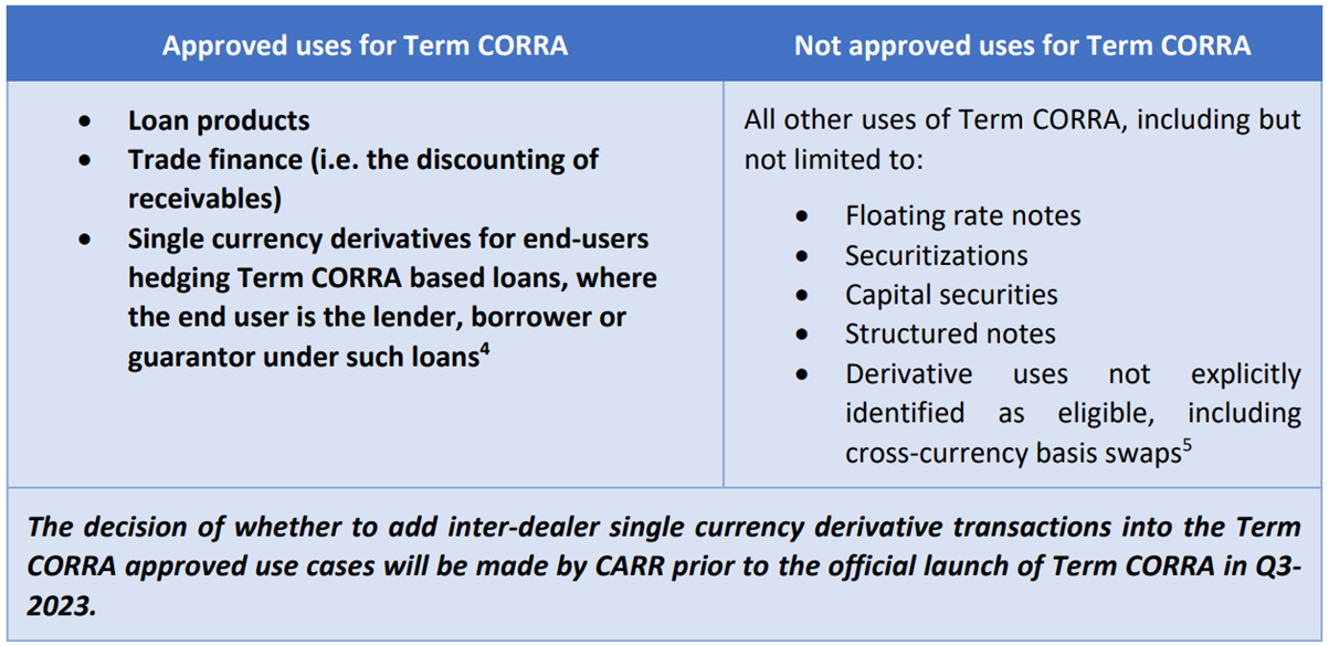
And understanding the Use-Case Limits
As I explored last year in Term RFR use limits; what use are they?, if use-case limits are here to stay, firms should start considering the use-case environment and their response quite carefully:
Ensure that use-case controls prevent dealing activity that contravenes regulator or industry preferences, and/or licensing requirements.
Establish a rules-based exceptions mechanism for allowance of Term-RFR use where use is warranted, and processes that document and track artefacts where use-case exemptions are approved.
Understand the peculiar reset risk that exists where Term-RFR’s are hedged via traditional OIS products.
Define and tag Term-RFR products as such, including within risk systems where unexpected basis and reset risk can emerge (between Term-RFR and traditional OIS hedges).
Ensure key staff understand term rates, their role in finance, their use-case limits, particularly where such staff are customer facing.
For Canadian-dollar risk, we would add that it will be important to understand the subtle variation that CARR has flagged already:
This appears to open up the possibility that a Canadian term rate could trade in interdealer markets, though how that might be ‘policed’ is another matter.
To our mind it would be better if the wish list of CARR’s Canadian respondents were met fulsomely, and preferably with a generous relaxation of use-case limits – a topic which we intend to explore in greater detail through 2023.
Summing up
Canada continues to surprise markets with the evolution of CORRA, and now a Term-CORRA benchmark solution. This is in a helpful alignment to developments in the US, where CME Term-SOFR activity continues to develop apace.
Other jurisdictions should be thinking about the market infrastructure developments that the Canadians see as crucial building blocks for finance and financial markets in an IBOR world.
From where we sit it really is hats off to the Bank of Canada and their Canadian Alternative Reference Rate Working Group.
Challenges in using SOFR for all loans
Bank funding risks

Many of our clients are asking about the impact of using risk free rates such as SOFR and SONIA in loan products which allow for discretionary drawdowns. This is especially challenging in the case of revolving credit facilities and particularly those with multi-currency options.
The choices of when, how much and which currency a bank can allow a borrower client to draw down in certain products has always been a challenge to manage. For example, in times of significant stress (e.g., GFC and COVID) the clients can suddenly draw cash from revolving facilities which can create liquidity and pricing problems for the banks.
In the past, the pricing of these facilities was somewhat easier because the reference rates were intrinsically linked to credit-sensitive benchmarks such as LIBOR. When liquidity and credit was stressed, LIBOR typically rose faster than Fed Funds (i.e., the TED spread increased) and the pricing of the loan facilities reflected the increased cost for the banks. This was automatically transferred (in the most part) to the borrower as the reference rate (LIBOR) closely tracked the bank’s borrowing rate.
This affected the bank profitability, the cost of the loans based on that expected cost/return and the behaviour of the borrowers. Banks could reasonably accurately price the facility based on expected costs (additional spread) and borrower drawdowns (expected liquidity requirements) and so were generally prepared to offer competitively priced products to clients.
The recent paper published on 22 December 2022 on the Federal Reserve of New York site and authored by Harry Cooperman, Darrell Duffie, Stephan Luck, Zachry Wang, and Yilin (David) Yang looks at the possible costs and therefore pricing challenges for banks when using SOFR rather than LIBOR for certain loans.
For those whose holiday calendar resulted in them missing this important paper, I really urge you to read the full transcript. In the meantime, I will outline some of the main points and my view of how these may impact banks and their clients.
One word of caution: the authors do note that the paper does not necessarily represent the views of the NY Fed or the Federal Reserve.
Bank Funding Risk, Reference Rates, and Credit Supply – Federal Reserve of New York – 22 December 2022
The paper references some very interesting data and does some really great analysis. The work focusses on the revolving credit loans that give borrowers the option to draw funds up to the credit limit at any time under agreed terms and pricing.
These credit facilities are widely offered by banks and are often used by their clients to guarantee funding for short periods of time even when liquidity conditions in the broader market may be challenging. It is this optionality and the very real likelihood that clients will require the funds at short notice in difficult markets that dictates the terms and pricing of the facilities.
The facilities tended to use credit-sensitive reference rates (e.g., LIBOR) which reflect the actual borrowing rates for the banks at a point in time. In this case, the underlying market conditions are automatically included in the LIBOR pricing for the clients and the banks can offer these products at competitive prices and terms.
The authors look at the impact of replacing LIBOR with risk free rates such as SOFR. They run some simulations for GFC (2008) and COVID (2020) and compare the performance of the products (LIBOR plus a fixed credit spread versus SOFR plus a fixed credit spread).
Without the credit sensitivity (i.e., using SOFR), the banks would be very likely to have a lower margin (NII – Net Interest Income). This was particularly evident in GFC (-6.48 billion) while the COVID experience was lower (-1.59 billion).
This is demonstrated in the following chart used by Ross Beaney previously.

These results can be found in Section D of the paper – Accounting Counterfactual Assumptions & Additional Results, Appendix D.
Why does this matter?
The authors conclude that the choice of reference rate (LIBOR or SOFR) affects the supply of revolving credit lines.
Under LIBOR referencing facilities, the bank and the client share the embedded liquidity risk. As the market supply of funds decreases, the cost increases (i.e., LIBOR rises relative to Fed Funds) are largely passed on to the borrower. The lender (the bank) still retains some risk as their individual ability to borrow funds from the market may be impacted by their own credit compared with other banks and this may diverge from LIBOR.
Point 1
This could result in the banks increasing the pricing for revolving credit facilities linked to SOFR or restricting the supply of these products. Because the risk is now firmly with the bank, the pricing and supply must reflect a ‘worst case’ scenario where the bank has limited ability to borrow from markets and/or an increased cost.
Note that this is not such a major issue for standard, term loans. These products can be term funded at a known margin and do not have the optionality for drawdown. In this case, there is little or no uncertainty about the principal and timing of the drawdown and repayment of the loan.
The authors do not consider multi-currency revolving credit facilities in their work. In my experience, the multi-currency option creates even more issues for banks and their clients. If you use a credit sensitive reference rates for the optionality within one currency (e.g., AUD BBSW) and a risk-free reference rate for another currency (e.g., USD SOFR), then under certain market conditions, one alternative could be far better than another for the borrower. For example, with a fixed spread to SOFR, if the actual market rate is above SOFR plus the fixed spread, then the rational borrower would logically opt for the USD.
Point 2
Multi-currency revolving credit facilities present additional problems for pricing and supply of the product. A bank must reasonably use the worst-case spread for a risk-free rate or risk being drawn on the facility when liquidity spreads exceed the fixed spread in one or more currencies referenced in the facility.
Is there another way to resolve this?
Fortunately, several credit-sensitive alternatives exist which could be used to replace LIBOR and be used with or instead of SOFR. We have previously written on this subject here, here, and here.
In the USD market these include:
Across the curve Spread Indices – SOFR Academy and Invesco
Bloomberg Short-Term Bank Yield
Credit Inclusive Term Spread/Credit Inclusive Term Rate – S&P Global – not yet available for licensing.
Published by AFX
I will not describe each of these alternatives, but the links are provided for further information if you are not already familiar with the reference rates. In all cases, they have reasonably tracked LIBOR in the past and add back a level of credit sensitivity.
If Messrs Cooperman, Duffie, Luck, Wang, and Yang are correct in their conclusion that SOFR-linked revolving credit facilities may be affected (I.e., negatively compared with the outgoing LIBOR equivalents), using the newer credit-sensitive rates above may help restore the risk balance. This may allow the banks to continue to offer these products as they do now.
Summary
The 22/12/2022 paper (and I appreciate the alliteration!) highlighted some particularly important challenges in the transition from LIBOR to SOFR for revolving credit facilities. The authors rightly point out that pricing and supply of these facilities may be negatively impacted.
While they did not look at multi-currency facilities, these present even more problems for banks who now provide these to clients.
Many end-user borrowers have such facilities to ensure they can have liquidity available under all circumstances. They may be expensive but are essential components of good risk management for many corporate and investor firms.
If the supply and/or price of these products is negatively impacted, there is a real risk that the end-users may face increased risk to liquidity crises in the future.
ESG maturing, far from settled…
We have been asked on several occasions whether we believe ESG-Investing has reached a state of reasonable maturity in capital and financial markets?

On each occasion I have proffered a rather hurried and wholly inadequate answer in the negative. In this blog I attempt to address this by cataloguing evidence of where greater maturity and/or standardisation is needed.
By way of reminder, Martialis takes no sides in the question of whether ESG investing adds value. If there is a value-assessment debate it is for others to determine, though we view the ultimate goals as laudable.
What follows should not be considered complete. While I have attempted to filter objectively, the starting point for the catalogue is inevitably opinion-based, or based on our experiences, and as usual – everything is contestable.
Some fundamentals
Let me start by making two general observations on the question of whether matters-ESG are ‘settled.’ This is a somewhat different question to whether they are, as yet, mature.
Firstly, modern investing owes much to the earliest open-air markets that started to evolve in and around the Warmoesstraat in Amsterdam in the late 15th Century. In their seven hundred-plus years evolution various approaches to investing have advanced and diversified, but never settled. Hence, at this relatively early stage, we should expect the ESG-investing domain to likewise advance and potentially diversify over time.
Secondly, while the world’s capital markets are truly enormous, it’s not clear whether there are sufficient ESG-rated securities to meet demand at any point. For example: if the world’s savings pool were directed entirely at ESG-rated assets above a certain score, their availability would be an obvious limitation. This is also food for thought for those who might be concerned at prospective concentration and/or asset hoarding risk (a topic for another day.
With this aside, I focus on reasonably objective areas that demonstrate that more mature ESG investing environment remains ahead of us.
The catalogue
John Feeney’s recent blog underscored the benefits of industry standardisation in benchmark setting, noting that:
“Markets depend on a level of benchmark standardisation that makes each dealer and end-user confident of the performance and valuation of each product.”
And:
“Most deep and liquid markets depend on a standard benchmark for risk resetting which is widely available and used in the majority of traded products.”
While John was pointing to the benefits across traded products, I think it is reasonable to extend these contentions to global finance more generally.
What we know is that in domains such as, say, transport, standardisation that turned cargo freight into uniform cargo in the form of ISO-standardised containers and pallets has driven incredible efficiencies. We can also agree that in financial markets high degrees of homogeneity have dramatically improved the efficient movement of capital between economic agents.
Thus, the catalogue that follows leans heavily on our enterprise view of the attractiveness, benefits, and likely efficiency-gains of adopting highly standardised and transparent approaches in markets:
ESG Ratings
Whereas the credit rating domain settled around a group of core agencies with well-understood approaches and ratings actions, the ESG ratings space continues to evolve.
As John noted, ESG evaluation criteria vary between multiple different rating platforms and are typically not independently verified, thus there is “no existing robust and standardised measure of ESG which captures a wide range of inputs and could be classified as a financial benchmark.”
Separately, it’s reasonably clear that ESG ratings are themselves an emerging specialisation, evidenced most recently in the unfortunately high ratings achieved by FTX on governance measures by a prominent ESG ratings firm.
Investment managers should note that ratings and ratings standards are neither fixed, nor a one-way bet.
2. Pricing (particularly sustainability premium or ‘greenium’)
We would normally view pricing as the rather obvious interaction between buyers and sellers known as price discovery in transparent markets, but this is a feature of mature markets. In less mature settings the pricing of individual deals may be shrouded by ‘tailored estimation’ (in the absence of an observable markets), and price discovery may be problematic given the one-sided nature of demand.
And this appears to be the case with ESG deal price-setting.
We note that in a recent ISDA survey, The Way Forward for Sustainability-linked Derivatives, the association asked members how ESG premiums are determined. Of 69 survey respondents a clear majority (45) indicated they “did not know how these premiums are determined.” ISDA also referred to the SLD market (sustainability linked derivatives market) as being “nascent” and described the sustainability premium or “greenium” as a “new concept in derivatives trading.”
These are obvious features of illiquid or partially formed markets such as those found in the price of highly complex derivatives.
3. Primacy
Corporate finance valuations have generally advanced down return or risk-compensated return dominant pathways. This was the logical advance of finance theory driven by advances in thinking around CAPM models and the like, aided by return-based concepts such as RoIC, RoCE, and RoE and broader economy concepts such as those found in the macroeconomics field.
While the layering of ESG filters within investment processes can take many forms, the question of ESG primacy arises. At what point should ESG filters be applied? Is there a fixed line, or some flexibility? What of exceptions? Should ESG factors take precedence, before traditional valuation approaches are applied?
We note that there are a variety of approaches being taken among clients, and other investment entities with whom we are close. Few are attempting a strict Blackrock ETF-like approach, though all have found themselves under pressure to respond in some fashion.
4. Portfolio Construction
Portfolio construction and asset allocations are considered by many to be at the heart of investment management performance.
Linked to the question of ESG-primacy is the question of whether a filtering process (particularly very strict approaches) may have unintended consequences in terms of optimal portfolio construction?
This is an emerging yet important topic. Is a traditionally risk-efficient portfolio, one suited to one or more beneficiaries under traditional allocation approaches, corrupted when ESG filters are applied (particularly if stringent filters remove whole sectors from consideration)?
There are a range of views on this, and I do not propose to dig into them here, however, we note that ESG scores for certain investable sectors are more readily achieved than in some others. At a minimum, we would expect this to have a bearing on portfolio concentration (and this may have played-out across the sweeping return-themes of 2022, in the dramatically skewed returns to energy sectors compared with new-economy stocks).
5. Emerging Standards
Perhaps the greatest area driving ESG towards maturity at present is that of the impending transparency, particularly in the sustainable finance edge of ESG. We see this as being driven by a range of government and regulatory agents.
There are simply too many global initiatives in-train to mention at present, but by way of example:
Australia - National Sustainable Finance Strategy,
We view these as likely to shape and enhance ESG maturity by bringing a degree of standardisation, but this will take time.
In this sense such initiatives are to be welcomed, but they are not yet embedded or systematically applied. They are also occurring on a multi-jurisdictional basis, and though we can acknowledge the work of the UN, there appears to be only vague international coordination.
We urge investment managers to watch these developments closely, since differing or changing standards can have a bearing on portfolio composition considerations.
6. Fiduciary Risk
We covered this topic in my blog of November 9th; ESG & Mandate Risk, which received reasonable interest and viewership. Judging by the number of follow-up engagements on the topic we expect the fiduciary question to linger.
Opinions certainly vary among readers as to whether fiduciary risk rises or falls away, but this itself is a sign that the question of fiduciary responsibility is not entirely settled. It may also be prone to shifting political sands on a jurisdictional basis (down to state level in the US as one example).
More recently, we have seen additional thought pieces on this topic appear, for example, Does ESG investing have a problem with fiduciary duty?, and related news that demonstrates there is a distance to travel before maturity is reached:
We continue to assess the various risks within this space.
Summing up
To sum up, we have been taking stock of the ESG domain for considerable time and have had several interesting client engagements on the topic. Much of what I have expressed here has been driven by such engagements, which have been highly productive and somewhat illuminating.
Our role is always to consider what is happening and be in a position to help inform decision-makers as their navigational needs arise, and as they ask where they should be positioned as events unfold To this end, it is helpful to be challenged on any topic, but on the question of how mature the ESG domain is for investment managers this has been very much the case, and we expect the challenges to continue.
While we are inclined to point out that there is a potentially long way to go, we can at least note that ESG investing is maturing but not yet settled.
As always in finance, some complexity remains, and market participants will have to keep adjusting.
Trading ESG Risk
Deep and liquid traded markets
Many financial risks can be acquired or modified through trading of securities and/or derivatives. For example, derivative products related to interest rates have been traded for many years and has seen the considerable growth of markets to shift risk from firm to firm. An active market to trade the risk has enhanced the ability of investors and borrowers to settle on the type and amount of risk best suited to their needs.
Another example is equity risk which also have deep and tradable markets. In this case, derivatives often reference an index such as Dow, S&P500 and NASDAQ which allow participants to trade the general direction of the market or alternatively trade sectors or even individual names. In each case, the underlying floating rate or index is clear and readily referenced to benchmark the trade.
Markets depend on a level of benchmark standardisation that makes each dealer and end-user confident of the performance and valuation of each product. Even the much-maligned LIBOR played a pivotal part in the development of traded interest rate markets. Without a standardised measure for risk setting such as LIBOR, derivative markets, for example, would have been impossible to trade in such a simple and definable way. And as LIBOR was replaced by Risk Free Rates such as SOFR and SONIA, the traded markets have adapted and continued to grow.
Likewise, equity markets have developed effective benchmarks for pricing in markets and allow for efficient risk transfer.
Most deep and liquid markets depend on a standard benchmark for risk resetting which is widely available and used in the majority of traded products.

The ESG markets – the next frontier
The ESG markets do not, at present, have the ability to trade the ESG risk in an equivalent way to interest rate or equity risk. There is no inter-dealer ESG derivative market and no standardised rate or benchmark to reference in a similar way to interest rates or equities.
A few firms do produce ‘ESG Scores’ which are not, technically, benchmarks. These include:
rating agencies such as S&P, Moody’s and Fitch;
Data providers such as Bloomberg and Refinitiv; and
Others such as ISS, MSCI, Datalytics etc.
While these agencies and vendors produce a ‘score’ from publicly available data (such as annual reports from companies) they are quite clear that these are not independently verified. In this sense, they are not benchmarks and could not be used under the regulatory requirements of many jurisdictions for the purposes of a benchmark, I.e., typically defined as refixing a variable rate or valuing a security.
So, there is no existing robust and standardised measure of ESG which captures a wide range of inputs and could be classified as a financial benchmark.
Why does the lack of a benchmark matter
If you have a risk or a desire to trade a financial product, you usually look at a screen where the bids and offers are posted for the products in which you have an interest. The products have standards and definitions which are supported by contracts and documentation such as that provided by ISDA for derivatives.
Whether it is a swap for fixed against floating or a fixed rate security, there is a need for an index or benchmark to provide the floating side of the trade and/or the valuation of a security. This is at the very heart of ‘price discovery;’ itself an important efficiency-driver.
It is particularly useful to use a standardised benchmark for obvious reasons. Once the benchmark is defined and readily available then there is a consequent reduction in the complexity of the trading because everyone is referencing the same rate or index.
Without a standardised benchmark, ESG products are difficult (I.e., near impossible) to trade in the inter-dealer market which means everyone simply builds up risk with no effective way to trade this into a market where the other side may be found.
One-sided or two-sided markets if an ESG benchmark can be developed
There is a market view that any ESG market would only be a one-sided (i.e., everyone wants to receive ‘fixed’ and pay ‘floating’ ESG). It is likely the result of the rush into ESG exposure and the perceived lack of floating rate investments that seems to drive this argument.
However, I take a slightly different view. Let’s take the example of a company with a debt linked to ESG performance. These have been transacted where the margins on the fixed or floating debt reduces as ESG performance improves (however that is measured!).
In this case, if the company had assets with fixed returns, then they may be a natural fixed rate payer of the derivative to match the asset risk to the liability risk. So why have ESG linked debt? Well, investor demand may be such that ESG debt represents cheaper funding, but it needs to be swapped for better risk management.
The investor argument is also important. Not every fund is ESG focussed, and some investors may actually need additional non-ESG exposure if they can only acquire assets with ESG links in the names they need for diversification.
I am a believer in traded market efficiency. If there is a market which is clear and standardised, a basis may form but equally the arbitrageurs will move in if that basis is unfounded. Price discovery is fundamental to their work.
Summary
The ESG market is growing and evolving as borrowers and investors respond to changes in demand. The current products are generally customised and structured for individual needs and are therefore not easily tradeable.
For deep and liquid markets to develop, there will need to be considerable development of standards and documentation for products (see ISDA survey) and credible benchmarks to support the products. While there are some ‘scores’ available there are no robust benchmarks to apply to products.
Along with the products for borrowers and investors, a supporting derivative market is essential to allow firms an efficient way to move and diversify the risk. A derivatives market needs a benchmark, and this is one of the major components of the market yet to develop.
ESG & Mandate Risk
Recent events in various US jurisdictions have highlighted an important set of questions around ESG investing. We believe these need to be considered by those holding a position of trust in the management of investor funds. Specifically, questions have been raised publicly about the nature and form of mandates governing the actions of funds.
In this blog we take no sides in the question of whether ESG investing adds value. Instead, we take a closer look at questions related to investment mandates under ESG and find that it may be worth those with fiduciary responsibilities taking their mandate into full and frank account.

Recent Challenges
Environmental, Social and Governance – ESG - investment platforms made unexpected headlines in the United States through Q3.
This included certain reports.
19 US state attorneys general wrote to BlackRock, arguing that the investment manager’s ESG investment policies may violate the ‘sole interest’ rule, which in the US requires that conflicts of interest in fiduciary relationships be avoided.
Attorneys General in Indiana and Louisiana issued warnings to their respective state pension boards that ESG investing may be a violation of their fiduciary duty.
West Virginia barred Blackrock, JPMorgan, Goldman Sachs, Morgan Stanley and Wells Fargo from contracting for new business in the state after determining that through ESG policies they were boycotting the fossil fuel industry.
Texas identified 10 companies, and 348 investment funds whom legislators labelled ‘boycott energy companies’, including BlackRock, Credit Suisse and UBS, prohibiting them from contracting with state agencies and local governments.
Our attention was drawn to this by a recent Wall Street Journal piece which noted that the principles invoked in the letters sent to Blackrock are “part of the common and statutory laws of almost every state.”
While it may be tempting to dismiss the Journal’s authors as partisans assembling contestable assertions, see here and here, we leave the tactical debate to others, for example:
Harvard Business Review:
o Yes, Investing in ESG Pays Off; versus
o An Inconvenient Truth About ESG Investing,
What we find interesting is that:
The various state-based challenges reignite a debate around fiduciary responsibilities that emerged when Corporate Social Responsibility, started to emerge in the early 2000’s; and, more importantly
ESG investment may be argued to contravene the Uniform Prudent Investor Act, adopted by 44 US states and the District of Columbia, which states:
No form of so-called "social investing" is consistent with the duty of loyalty if the investment activity entails sacrificing the interests of trust beneficiaries – for example, by accepting below-market returns -- in favor of the interests of the persons supposedly benefitted by pursuing the particular social cause.
The Journal’s writers, William Barr and Jed Rubenfeld, go on to note that “a defence to ESG investing asserts that ESG factors, though nonpecuniary, are material to profitability and that ESG investing will therefore produce superior outcomes.”
This appears contestable, as the varying Harvard studies amply prove, but when canvassing for views from among Martialis clients and contacts one message stood out: most managers have been inundated with requests for ESG-overlay and careful observance, not the opposite.
Fiduciary Duty in Australia
We hope to follow up on this blog with a more detailed look at the nature of fiduciary responsibilities in an Australian context. The aim will be to get a much clearer definitional picture from experts, so watch for that in coming issues.
What we do note is that there appear to be similar provisions within the Corporations Act to those written-in to the US’s Uniform Prudent Investor act. For example, a responsibility under the Australian Act is that responsible entities (of registered schemes) duties include acting “in the best interests of the members and, if there is a conflict between the members' interests and its own interests, [to] give priority to the members' interests."
Perhaps the risk for fund directors lies in the definition of what constitutes a member's interests? Is it to maximise returns with an ESG filter or overlay, or simply to maximise returns?
In our view, risk here can likely be distilled into to a fundamental question of fund mandate.
Where a fund has ensured beneficiaries are aware of the nature of the decisions being made – whether ESG-based or otherwise – a mandate sets the parameters within which a portfolio is managed, thus setting properly informed beneficiary expectations.
But what of funds that have started overlaying ESG filters without addressing beneficiaries or their mandate?
To us, this seems problematic.
A problematic greenium
As the market transparency of ESG investing modes develops it will be increasingly easy for fund beneficiaries to assess the decision-making path of fund managers.
To reinforce this, we note that Bloomberg has embarked on an extensive ESG program designed collect some data to the ESG metrics.
Bloomberg’s Environmental, Social & Governance (ESG Data) dataset offers ESG metrics and ESG disclosure scores for more than 14,000 companies in 100+ countries. The product includes as-reported data and derived ratios as well as sector and country-specific data points. In addition to the extensive ongoing data coverage, we provide historical data going back to 2006.
This allows Bloomberg subscribers to gain access quite remarkable decision-making tools and transparency.
For example, here is a screenshot of Bloomberg’s Green Instrument Indicator:
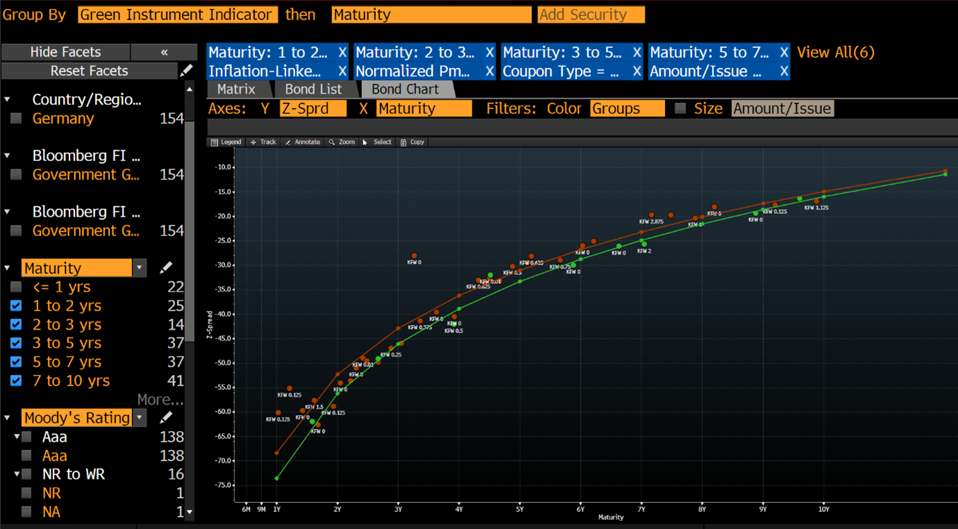
Which means that transparency is assured.
What then of a situation in which, for example, a bond fund manager is considering a purchase of bonds/bunds of, say, a noted green issuer - the Federal Republic of Germany?
The German state issues both green and non-green bonds, and has gone to impressive lengths to distinguish between the two:
The use of proceeds from Green German Federal Securities always corresponds to federal expenditure from the previous year. Spending from the previous year’s budget that qualifies as “green” is assigned to the securities. The Green Bond Framework lists five main green expenditure categories that can be assigned to Green German Federal Securities.
These are:
Transport
International cooperation
Research, innovation and awareness raising
Energy and industry
Agriculture, forestry natural landscapes and biodiversity
Noting that the yield differential between a 10-year green and traditional bund is around 5.0 basis points, it’s not hard to see a potential fiduciary risk problem emerging.
If our bond fund manager notes the differing market yield representing the ‘greenium’ (which we imply as resulting in a lower monetary yielding outcome for the investor) and has no mandate for such a product we suggest there is a potential problem.
Why?
Because a beneficiary who considers their best interests to be served by owning higher yielding paper – irrespective of their views of ESG outcomes - could make the argument that the manager was in breach of their fiduciary duty. Transparency makes their argument much easier.
Which brings us back to the question of fund mandates, and several important questions:
· Is the fund mandate current?
· If mandate changes that were likely to diminish fund returns have been implemented, were beneficiaries advised of these changes?
Those holding fiduciary responsibilities should take their mandate into full and frank account, or at least ask two questions:
1. Is our mandate current?
2. Is our mandate clear?
Summary
ESG investing is very topical among investors. However, the investment mandates are important documents which need to be observed. In addition, regulators and legislators are now taking interest in the investments and often taking action to protect their industries.
We will be writing more on this in the near future.
Variation and Initial Margin Collateral Management - A new challenge
1 September 2022 marked the introduction of the final phase of Uncleared Margin Rules (UMR). This has been a very long process which has included 6 phases and has gradually caused a large number of market participants to post variation and initial margin to support their derivative trading. It is worth noting that UMR only applies to new trades after the date of implementation.
In the case of variation margin (VM), most jurisdictions require ‘financial counterparties’ to exchange VM while generally allowing end users an exemption.
For initial margin (IM), if the Average Aggregated Notional Amount (AANA, which is basically the gross notional of all uncleared derivatives including FX) exceeds a specific amount at each phase, then both counterparties are obliged to post IM for their uncleared non-FX derivatives if they are both ‘covered entities’ (i.e., have exceeded the AANA at any phase).
The implementation calendar is as follows:


Why is VM and IM collateral a challenge?
VM has been used for many years prior to 2017 as a credit mitigant to offset the mark-to-market (MTM) of a derivative with a counterparty. VM can be posted or received depending on the MTM.
IM is posted by both counterparties to independent custodians. It does not depend on the MTM, but rather on the risk of the derivatives. It is seen as insurance against future movements in MTM.
Changes to capital calculations for many banks (Basel I, II and III) have also contributed to the use of VM and IM. Where banks use collateral, they can reduce the capital drag on derivatives substantially, making them more competitive and increasing returns. This impact can also change the pricing of derivatives for end users as banks using lower capital can effectively ‘pass on’ the savings.
While IM Phases 1 – 4 had their own issues, the firms involved had significant resources and experience in managing and providing IM with each other for uncleared exposures and with CCPs for their cleared trades. The problems for these firms were often associated with engaging the independent custodian and setting up separate accounts. For example, in Phase 1 there were approximately 10 firms but they each required thousands of individual accounts at custodians to support the legal entities! All this took time and effort.
As we moved to Phases 5 and 6, the firms captured by the regulations are often less familiar with the operational requirements of posting IM and managing the complexities of posting and receiving VM. They also, like the previous phases, needed to set up custodian relationships and open accounts as necessary.
The number of Phase 5 and 6 counterparties is estimated at 1,200 in total which far exceeds the previous 4 phases (~100 in total). When the significant number of new firms and the probable level of experience of those firms is combined, there are challenges for all participants as there are 2 sides to every transaction with individual and joint responsibilities.
If there is a mismatch in capability and experience between the counterparties, there can be ongoing challenges for both counterparties in both VM and IM.
Challenge 1 – Agreeing and reconciling IM and VM
All regulatory jurisdictions require counterparties to agree the IM and VM amounts daily within quite tight tolerances. If the counterparties cannot agree, then a process of reconciliation commences.
This generally starts with checking the actual portfolio (number of trades) followed by valuations of individual trades (VM) and risk inputs to IM calculations. These activities can be complex, detailed and time-consuming. In many cases, sophisticated quantitative tools are required which may not be readily available to both counterparties. We have found that Phase 5 and 6 firms in particular do not have these tools and processes established and ready to deploy.
With short timelines for reconciliation, some clients are having problems achieving the short turnarounds required for resolving IM and VM differences.
Challenge 2 – Availability of acceptable collateral
Most firms who post or receive VM collateral have reviewed their documentation and restricted the options for that collateral to currencies and/or securities they can access for posting and accept when receiving. For smaller firms, this is often cash in their domestic currency as they have limited availability of foreign cash for posting and limited ability to accept and invest a foreign currency.
Although USD is the standard collateral currency, we have found many smaller, buy-side firms will require their domestic currency as VM. This does solve the operational problem but can create other complexities such as that in Challenge 4.
IM has a very different collection of potential issues. The generally preferred IM collateral is limited to certain types of securities (e.g., government bonds) which are agreed between counterparties and can be accepted by their respective custodians.
Larger firms (banks) can routinely access these securities either directly from their own accounts or via repo markets. Either way, they have established and efficient processes to find and post the required IM collateral.
Smaller firms typically do not enjoy the same access to these securities, especially investors who own other securities aligned with their investment mandates and return metrics. Cash is not preferred by custodians, and they will charge large fees for accepting cash as IM due to regulatory costs. Repo is available but firms still need cash collateral for the repo and the systems and processes to trade and settle the repo. Again, this is very costly and inefficient for smaller firms.
We have found that smaller firms have often had problems accessing and managing collateral especially for IM.
Challenge 3 – Balancing fund returns for investment firms
Investment firms have an additional set of challenges that arise from the multiple funds, legal entities and fiduciary duties associated with those funds.
Many firms need to maintain separation between the funds and accurately record and price collateral borrowed from one fund to post for another fund. This is fast becoming and issue for Phases 5 and 6 firms as they begin to post IM created by derivatives in one fund, but they borrow the securities from another fund. This has to be priced at arms-length and accurate records and accounting entries posted to maintain the integrity of each fund return.
Challenge 4 – Pricing and revaluation
USD collateral is the standard for pricing derivatives and the published prices are assumed to be using this standard. For example, a USD interest rate swap uses USD SOFR as the default collateral as does a USD/JPY or USD/AUD cross-currency swap. In the case of other currencies, the collateral is assumed to be the domestic currency, for example AUD interest rate swaps use AONIA as the assumed collateral return rate.
As outlined in Challenge 2, many smaller firms prefer their domestic currency. In the cross-currency example, many buy-side firms have VM in JPY or AUD depending on their location.
When you change the collateral currency assumption, this can (and often does) have an impact on the price of the derivative. In some cases this difference is small and can be effectively ignored. But in other cases (e.g., cross-currency) the impact can be significant and can change the price.
All firms need to be able to price this difference: either they are charged for it or they need to demand the better price. Otherwise, a sophisticated, unscrupulous counterparty may simply ‘trouser’ the profit and the less aware firm will never notice the difference.
So, what you see on the screen as the price of a derivative for a new trade or a revaluation rate may need to be adjusted for your collateral currency if it is not USD or the assumed domestic currency for that derivative.
Revaluation rates are also problematic for many firms as they must adjust the rate from a screen or valuation service to reflect their collateral arrangements per counterparty. This is very complex and can seriously impact both accounting and the ability to reconcile VM and IM with a counterparty.
Challenge 5 – Back testing the portfolio
Firms included in all IM phases in most jurisdictions are require accreditation by their local, and occasionally offshore, regulatory authority. One of the more difficult and ongoing challenges for many firms is demonstrating appropriate back testing of the portfolio to show the IM posted is adequate to cover the risk of default.
Banks have been doing this for many years with VaR and stress testing requirements. But non-banks have typically not had this form of reporting obligation until they became ‘covered entities’ for IM.
The back testing is usually done daily, and regulators want to see rigor and maturity in testing over a certain period in the recent past and stress tests to cover extraordinary events. This is overly complex and is often a new process for many non-banks.
Our recent work has shown that many firms are finding the technical and operational aspects of back testing difficult to implement. The choice and maintenance of stress events is similarly challenging as it relies on expert judgement to find the appropriate scenarios for their own portfolio.
Summary
Collateral is now part of doing business for many firms, either through regulatory obligation or increasingly through counterparty requirements. Whether using clearing services (i.e., CCPs) or uncleared bilateral relationships, collateral is an important consideration for many firms.
We see the number of firms using collateral increasing and the complexities of managing the operational and technical challenges can be new and significant for many of them. The challenges can be managed with careful planning and some essential tools.
We have listed 5 challenges above but there are often many more. Each firm has their own idiosyncrasies with operational and technical improvements which are needed to manage collateral.
Why debate over credit sensitive rates won’t go away…

It’s not a debate being played out around weekend barbeques, and it’s not likely to gain regular billing on 6 o’clock bulletins, but the question of whether finance needs credit sensitive benchmarks is one we’ve looked at many times – and yes, debated.
In my latest blog post I look at a rather obvious pitfall that seems likely to arise if corporate finance doesn’t settle on a credit sensitive lending solution.
Urban Jermann
Urban Jermann is Safra Professor of International Finance and Capital Markets at the Wharton School of the University of Pennsylvania. In December 2021, Professor Jermann released a topical research paper titled: Interest Received by Banks during the Financial Crisis: LIBOR vs Hypothetical SOFR Loans, which was a formal study into the cost to the US banking sector that might have been incurred (interest earnings foregone) had US business loans been indexed to SOFR reference rates (instead of LIBOR) during the two years of the GFC.
Jermann’s work is interesting from several standpoints:
He uses the expression “insurance payout” to describe the credit sensitive component of the lift in LIBOR rates through the GFC, which is both interesting and, in our view, a healthy development since banks may like to consider actuarial approaches in assessing their long run risk to credit sensitivity, and,
He calculates estimates of the “payout” LIBOR lenders received over what they would have had their loan books referenced SOFR in both compound and term formats.
He notes that:
The cumulative additional interest from LIBOR during the crisis is estimated to be between 1% to 2% of the notional amount of outstanding loans, depending on the tenor and type of SOFR rate used.
And the amounts estimated that would have been forgone by banks on loans whose economy-wide balance “may have been as high as $2trln” are meaningful:
U$32.1 billion if loans had instead followed compounded SOFR; and
U$25.0 billion had they instead followed Term SOFR.
It’s important to note, these numbers are the hypothetical reduction in interest income US banks would have borne if loans had been struck against compound or term SOFR, instead of LIBOR between June 2007 and end June 2009, and incorporate the quantum of the following US loan-types:
Syndicated loans;
Corporate business loans (bilateral),Noncorporate business loans;
Corporate Real Estate loans
Professor Jermann obtained his data from the Shared National Credit (SNC) Program for syndicated loans, and the Financial Accounts of the Federal reserve for the other categories.
All of which unearths an important question: does the loss of LIBOR’s insurance-like credit sensitivity reduce banking sector returns if not compensated?
Our answer is probably, but not if average bank funding costs settle below their long run spread to risk-free rates and stay there indefinitely.
Which makes us wonder what kind of numbers Professor Jermann might have found had he chosen to analyse the post-GFC environment since major bank funding mixes been altered so dramatically in the aftermath of the GFC?
We think it’s also interesting to note that the interest foregone by banks would have been worsened under compounded SOFR compared to Term SOFR.
Credit sensitivity since the GFC
The post-GFC numbers are relatively easy to calculate, and while we’re not going to attempt to research the quantum of loans financed through that period, we will use post-GFC USD LIBOR/SOFR OIS spreads to estimate the potential loss in basis points per annum.
We find that mean and median loss of credit sensitivity as follows:

In other words, the average annual loss of credit sensitivity yield since the end of the GFC (June 30th, 2009), was 21.4 basis points (BP) for USD facilities.
Market anecdotes
Our most recent market soundings indicate that in loan markets in the US and elsewhere lenders are:
increasingly moving towards CME (Chicago Mercantile Exchange) Term-SOFR as the basis for new USD deals, in a clear move away from compounding;
that there is no clear consensus on credit adjustment spreads (CAS); and
that lenders appear to be simply adjusting credit margins where they can do so.
By the way, this latter practice results in the same outcome as lenders negotiating a fixed CAS and simply adding this to compound or term SOFR, i.e., analogous with the basic mechanic used in the ISDA (International Swaps and Derivatives Association) Protocol for derivative transitions.
The key point is that lenders who adopt this approach are fixing the credit sensitive component of the facility, and therefore foregoing the potential “insurance payout” of a credit sensitive alternative.
Our point is (and has been) that this practice may prove problematic depending on the extent to which recent credit spreads are reflective of future.
A long-term 3-month LOIS (LIBOR/OIS spread) proxy
To prove the possible problem, we have constructed an indicative 3-month USD LOIS proxy based on an adjusted TED-Spread (3-month USD LIBOR less Treasury Bill yields) going back to 1986.
It supplies an interesting picture of the peaks and valleys of a proxy credit-sensitive rate going back well into the distant years of modern finance.

The long run statistics on the proxy are as follows:

But we think it’s important to consider the historic levels of the proxy across differing periods and differing credit environments to prove how times can change; hence we have broken the data into 5-year periods to give a perspective based on different historic periods:

This approach shows that based on 5-year bucket analysis, banking sector credit was more expensive than the ISDA 3-month spread (26.15 basis points) in all prior periods and has been relatively rarely below the mid-20s.
It also appears somewhat correlated to the general level of interest rates, which makes intuitive sense. This should give those in favour of static CAS pause for thought (a possible topic for a future blog).
AXI has gone live
Which is why we can’t see the credit sensitivity debate disappearing anytime soon.
It’s also why we took a keen interest in the recent official release of Invesco Indexing and SOFR Academy’s Invesco USD Across-the-Curve Credit Spread Indices (AXI):
The AXI and FXI indices are forward-looking credit spread indices designed to work in conjunction with the Secured Overnight Financing Rate (SOFR).
AXI and FXI work to form a credit-sensitive interest rate when used in combination with Term SOFR, Simple Daily SOFR, SOFR compounded in arrears, or SOFR Averages.
AXI is a weighted average of the credit spreads of unsecured bank funding transactions with maturities out to multiple years.
The relevant methodology can be found here.
AXI’s release joins BSBY, and IHS-Markit’s USD Credit Inclusive Term Rate (CRITR) & Spread (CRITS), in the credit sensitive reference-rate stakes.
In conclusion
It’s impossible to accurately predict which mode markets will eventually settle on, fixed estimates, or dynamic credit. Our hunch is that credit sensitive rates will become an economic necessity once the unprecedented recent compression of financial market spreads and interest rates abates.
The use of fixed spreads based on recent LOIS history could be thought to weaken the overall financial system, since it’s hard to see how the lost revenue of Professor Jermann’s “insurance payout” gets made up for in any repeat of GFC-like credit conditions, but we are not forecasters.
There is, though, the possibility that like El-Nino and La-Nina we have recently traversed a period of an unusual credit risk drought in what is a cyclical system. In that case credit sensitivity should be considered of long-run benefit.
If banking serially misprices its own costs, there can be few actual winners.
Term SOFR – Moving forward because the demand is real
We have posted quite a few blogs on this subject, notably in May 2022 and April 2022. When these blogs were published, the use cases for Term SOFR very restrictive and are defined by the Term SOFR administrator (CME).

More recently, the ARRC has reconvened the Term Rate Taskforce which was reported in the July 13 Readout. The important aspect of this group’s work is to review certain aspects of the Term SOFR uses as in the Readout:
‘The Term Rate Task Force provided an update on its discussions around term SOFR derivatives. In particular, the Task Force has been discussing participants’ views on issues/questions around term SOFR derivatives and the overnight SOFR/term SOFR basis, including clearing, capital, and accounting considerations. It was noted, however, that the Task Force is distinctly not being reconvened to materially relax the substance of the ARRC’s best practice recommendations regarding scope of use for the term SOFR rate.’
The important word is ‘materially’. This implies some changes to the use cases could be supported and therefore able to be reflected in the CME licensing rules for Term SOFR. Risk magazine has covered this topic only recently (7 July 2022) and has provided insightful perspectives on what additional use cases may address participant requirements while still adhering to the basic ARRC principle of proportionality (i.e., not allowing exponential expansion of the use of Term SOFR to keep the volumes referencing the benchmark in proportion to the underlying transactions used to calculate it).
Current CME licensing
The CME website has the following data for Term SOFR use:

Licenses from the CME are divided into 3 categories:
Category One applies to cash instruments like loans, mortgages, bonds, notes, and money market instruments.
Category Two is necessary for applying Term SOFR as a reference in any derivative product. However, the catch is that the license only covers derivatives that are directly linked to cash instruments which reference Term SOFR.
Category Three is used by specialist providers in products or services they develop and license to external clients. We do not cover this category in the blog as it only applies to service providers.
The licensing for Category Two is quite restrictive, appears to create a one-sided market and excludes potentially compliant uses for Term SOFR. In practice, Category Two requires the derivative to only use reference Term SOFR if it applies to a cash debt exposure.
Why is Category Two restrictive?
Category Two, in practice, only allows for derivatives to be used to swap floating rates (Term SOFR) associated with cash products to fixed rates. In other words, a end user can only pay fixed and receive Term SOFR in a standard interest rate swap because the Term SOFR must be associated with the cash instrument to allow a derivative to reference Term SOFR.
One example where there may be an end-user use for Term SOFR is in a derivative swapping fixed debt coupons for floating USD. SIFMA does publish the corporate bond issuance statistics for USD as summarised in the following table:

The corporate bond market is large and a significant percentage (78 – 91%) issue fixed rate. A proportion of the fixed rate issuers may decide to swap the fixed coupons to SOFR and many of these issuers are possibly in a similar operational position to the issuers of floating bonds who are permitted to use Term SOFR.
However, the fixed rate issuers cannot access Term SOFR in the swap to achieve a floating rate liability as it is not allowed in CME Category Two licenses.
Is there any real difference between the floating rate and fixed rate issuers? Arguably there is no difference except the preference of investors at a specific time.
Perhaps there is a legitimate use case for corporate fixed rate issuers to use derivatives to swap to Term SOFR and therefore an amendment to the CME Category 2 licence may be appreciated to allow a fixed to term SOFR swap.
The challenge for the ARRC and the Term Rate Taskforce
The Term Rate Taskforce has been reconvened to consider changes to the recommended use of Term SOFR given how the market has evolved since 2021. (I very much respect their challenges in finding a way to balance the proportionality with clear end-user demand!)
One advantage of allowing for derivatives which swap fixed to Term SOFR is that it helps balance the current market where only Term SOFR to fixed rate is, in practice, permitted. This could remove or reduce the current additional costs of around 1.5 to 3.5 basis points for end user borrowers in referencing Term SOFR (see the Risk article above). I do note that investors could provide the balancing side of the swap, but they could just as easily buy floating rate products (as they seem to be doing in 2022!)
Should the use cases be expanded to allow for derivatives such as the example above?
Should there be inter-dealer trading (perhaps with some restrictions) to allow banks to clear risk and provide more competitive pricing for their customers?
We will have to await the outcomes from the ARRC, but the market is showing there is demand for a less restrictive approach to Term SOFR which would need to be reflected in the CME licensing arrangements.
Summary
While we have written blogs previously on this topic, markets have changed considerably, and the tensions are very clear. The Term SOFR derivatives market is currently one-way as reflected in the basis cost of swapping floating for fixed rate.
Allowing a more balanced market where end-users can have equivalent access to fixed to floating as well as floating to fixed swaps may address some of the pricing imbalances and also provide bank customers a more complete service.
If there is a (limited) inter-dealer market then risk can be cleared more readily and banks can move the Term SOFR exposures to their trading books, thereby reducing operational and capital costs.
There is a compelling argument that end users of Term SOFR derivatives would benefit from some adjustments to the ARRC-recommended use of Term SOFR.
I hope the ARRC can adapt the recommended uses for Term SOFR and that this will be quickly incorporated into the CME Category Two licensing.
CDOR, CARR, CORRA, CAG? What’s really happening in Canada?
The Canadian Alternative Reference Rate working group (CARR) was first established in March 2018 with a remit not dissimilar to the ARRC of the US Fed, to “guide benchmark reform efforts in Canada.”
In this blog I attempt to cut an explanatory path through the maze of acronyms that loom in Canadian finance, and distil what’s really going on with Canadian benchmarks, and try to gain a better understanding of the fundamental, underlying problem with CDOR.
Are there important lessons from the Canadian experience?

Why so many acronyms?
In every jurisdiction where benchmark reform has been attempted, new market acronyms abound.
This has been without exception, though we’d concede that the Bank of England Working Group on Sterling Risk-Free Reference Rates has seemed to defy market ‘acronymisation’!
Canada has been no Robinson Crusoe in this evolution, though the list of reform acronyms could be said to have been taken to new lengths in terms of sheer number. We’re sure this was not deliberate, but with so many new terms mixing with old terms it’s somewhat instructive to recap what they all stand for, and what role they play:
Canadian Dollar Offered Rate, CDOR, is administered and published daily by Refinitiv Benchmark Services. The rate was developed in the 1980s as the basis for pricing Bankers’ Acceptance supported credit facilities (short-term corporate promissory notes backed by an unconditional payment obligation of a bank). It has remained the primary interest rate benchmark in Canada since inception and is referenced in over $20 trillion of gross notional exposure across the Canadian wholesale financial system.
Canadian Alternative Reference Rate Working Group, CARR, was created through the sponsorship of the Canadian Fixed-Income Forum, to coordinate Canadian interest rate reform and “ensure Canada’s interest rate benchmark regime is robust, relevant and effective in the years ahead,” with objectives to:
o support and encourage the adoption of, and transition to, the Canadian Overnight Repo Rate Average (CORRA) as a key financial benchmark for Canadian derivatives and securities; and
o analyse the current status of the Canadian Dollar Offered Rate (CDOR) and its efficacy as a benchmark, as well as make recommendations on the basis of that analysis.
Canadian Overnight Repo Rate Average, CORRA, Canada’s official risk-free rate based on daily transaction-level data on repo trades that measure “the cost of overnight general collateral funding in Canadian dollars using Government of Canada treasury bills and bonds as collateral for repurchase transactions”. The Bank of Canada considers CORRA a public good and publishes rates at no cost to users and data distributors each business day at 11:30 am Canada Eastern Time.
CORRA Advisory Group, CAG, was initially established to advise the Bank of Canada’s CORRA Oversight Committee on potential adjustments to the CORRA methodology, “stemming from changes in repo market functioning and from any emerging methodology issues, as well as on any changes undertaken as part of regular methodology reviews.” A key role of CAG is to assess if CORRA continues to represent the overnight general collateral funding rate where Government of Canada securities are posted as collateral.
While to-date no formal Term CORRA rate has emerged, I note that Canadian industry demand for a CAD term rate is like that found in other jurisdictions (high, reasonable, and in our view very rational), and that CARR has a Term CORRA subgroup reviewing the need for “a complementary term rate to overnight CORRA for loan and related hedging products.” This welcome group is also expected to develop an appropriate methodology.
So, what’s the plan?
Similar to the approach taken in both the UK and US, and mirrored elsewhere, CARR has published its own well-laid transition roadmap.

Source: https://www.bankofcanada.ca/wp-content/uploads/2022/05/transition-roadmap.pdf
Readers with experience of the Bank of England roadmap to GBP LIBOR’s cessation will note the similarities:
announce a formal cessation trigger;
establish a ‘no new LIBOR (CDOR)’ exposure cut-off date; and
set a formal publication cessation date in stone.
We see no reason for Canadian markets to struggle with any of this, and market disruption should be minimal; the global template for cessation has essentially been set.
What’s the problem with CDOR?
Helpfully, CARR’s formal review of CDOR is available on-line, and I am leaning on it heavily through this section
After consulting with industry through 2021, and as outlined in the transition roadmap, CARR formed the view that Refinitiv Benchmark Services (RBSL) should cease the calculation and publication of CDOR after June 30, 2024.
My key question is, why was this?
CARR is explicit here, saying that “there are certain aspects of CDOR’s architecture that pose risks to its future robustness.”
What risks?
Here I paraphrase the two key risks CARR found, and which we believe are fundamental, to make summary easy:
Input rates crucial to CDOR’s publication cannot be directly tied to observable transactions, and are hence “based predominantly on expert judgement”. CARR decided that this was “not consistent with evolving global best-practices” nor, we would add, was this consistent with IOSCO Principles for Financial Benchmarks.
CARR noted that Bank funding has evolved to “better match the term of their funding to the term of their loans, and this practice is now codified in Basel III regulation”. Further, CARR noted that “BA loans are “term” or “committed” facilities, bank treasuries no longer fund them through the issuance of BA securities that are generated through the loan drawdown”. The reduction of bank acceptance issuance tolls a rather obvious bell.
CARR also noted that the move away from CDOR “aligns Canada with the heightened standards other jurisdictions began adopting in 2018,” and that the rate’s “contributing member banks may decide they no longer wish to continue submitting rates voluntarily.”
These are interesting other riders; hinting at a desire on behalf of the working group, and presumably others across Canadian finance, to follow the benchmark modernisation path seen across the US, UK, Japan, and Switzerland.
Boiling it all down?
When CARR tell us that “there are certain aspects of CDOR’s architecture that pose risks to its future robustness,” I am at once reminded of the fall in interbank (LIBOR) lending that has occurred since the mid-90s, and prominently since the GFC, as displayed in the classic St Louis Fed graphic on the topic:

Source: https://fred.stlouisfed.org
In Canada, the pattern has been familiar; bankers’ acceptances are simply no longer playing the significant role they once played in Canadian finance.
Short-term paper held on financial balance sheets has fallen to around 1% of the national balance sheet since Y2k:

Source: Statistics Canada. Table 36-10-0580-01 National Balance Sheet Accounts
Perhaps more interestingly, since the GFC short-term Canadian paper has hardly registered as meaningful liabilities on the non-financial sectors cumulative balance sheet either:

Whichever way CARR may like to couch it, dire levels of actual BA activity really has spelled the end of CDOR.
Important Lessons?
Our interest in Canada as a benchmark test-case stems from the similarities between Australian and Canadian finance, where bank accepted securities play and have played a key role in benchmark formation in both countries.
We will look more closely at the Australian benchmarks in the next blog.
Perhaps the most important lesson from Canada is that times change, and that rational actors will act rationally. Market evolution, some pushed along by natural market evolution, and some pushed along by regulators, needs to be carefully watched, and shouldn’t be ignored.
We continue to watch this space with deep interest.
USD Inflation – the barbed wire hedge
Ross Beaney posted a great blog on the Texas hedge which has attracted much interest. Ross provided the definitions for a Texas hedge as:
Oxford Reference Dictionary - The opposite of a hedge, which is intended to reduce risk. In a Texas hedge risk is increased, e.g., by buying more than one financial instrument of the same kind
Collins Online Dictionary - the opposite of a normal hedging operation, in which risk is increased by buying more than one financial instrument of the same kind.
He applied this to the Term RFR and compounded RFR markets to demonstrate the challenges of hedging one with the other.
Today I will look at the barbed wire hedge and I thank Andrew Baume for reminding me of this hedge variant in our LinkedIn post! So, what is a barbed wire hedge?
A definition for this unusual hedge is not available using the usual search methods on the internet because the term probably fell from common use in markets before the internet was ‘a thing’. My last recollection (before Andrew reminded me) was possibly in the early 1990’s and it was described as:
‘A barbed wire hedge is one where it does not matter which leg you lift to extract yourself from the risk and/or hedge, you are in trouble!’
The picture tells it all……….
In this blog, I look at the USD inflation markets and how the barbed wire hedge is an apt description for the challenges faced by many hedgers and the dealers who provide the prices.

Inflation history
The following chart is for the annual inflation printed in USD over the past 10 years. I use the annual data because it removes the considerable seasonal variations in US CPI and focusses on the actual trend.

There has been little or no trend until 2020/21. Everyone has noticed the increase in inflation in 2021 and 2022 which is clear in the chart above. We have had relatively low inflation for many years which has been broadly in at the Fed target of 2%. This can be seen in the next chart showing annual inflation outcomes since 1960 where inflation since 1995 has moved in a band between 0% and 4% oscillating around 2%.

But now we are close to 5% and trending up. Interest rates aside, what should we do to directly hedge our inflation risk? Will inflation peak this year as many expect? Or will inflation become more entrenched as we see happened from the mid-1970s to the mid-1980s?
I will not cover the possible causes for higher inflation in this blog but rather look at the challenges for hedging and what this can mean for hedgers and dealers.
Looking forward and inflation expectations
The following chart shows the 10-year forward USD inflation expectations over the past 10 years.

The markets clearly expected 10-year inflation averages to be around the 2% target until the COVID19 drop in early 2020 to a low around 0.5%. This quickly reversed as markets expected the US market to recover more quickly and priced in higher inflation.
The next chart shows the current, implied forward USD inflation rates (annually) for the next 10 years. The 10-year inflation swap is around 2.7% which incorporates the current expectation at 5.38% but the forward rates fall rapidly to 2% - 3% in subsequent years.

Markets are very clearly pricing a very transitory period of inflation followed by more ‘normal’ inflation rates around 2% after 2023/24.
The hedge challenge – the classic barbed wire hedge
With current inflation rates higher than in the past 20 plus years and seemingly trending up, there is an immediate decision for many firms to consider hedging. Or not.
Now, you are metaphorically astride the barbed wire fence. You hedge now and you lock in inflation at an average of 2.7% for 10 years with the implied rates in the previous chart. While this looks attractive, what if there is a recession and inflation returns to near 0% as it did in 2009 and 2020?
Or you could wait and see.
This also comes with a risk of a repeat of the mid-1970s to mid-1980s where inflation ranged from 5% to 14%.
Which leg do I lift first? Do I lift the hedge leg and accept the risk of higher inflation? Or do I lift the risk leg and lock in the current inflation curve? This is a classic barbed wire hedge conundrum where whichever decision you take, there are consequences, and you may wind up in trouble.
Summary
Decisions come with risks, but decisions must be made. The way forward for inflation is not as clear as it has been for many previous years where we had inflation expectations and outcomes around the 2% target. The current expectation is a return to the benign world of approximately 2% in the next year or so. But this may not be the case.
Whether you decide to hedge or not and whichever leg you decide to lift, there may be a time when you quickly need to reverse direction and replace the leg you lifted. To continue the analogy, when you are captured by a barbed wire hedge, take careful note of which leg to lift, manage the risks during and after the operation and be prepared to reverse if things start to go badly wrong.
Otherwise, the outcomes can be painful.
Of Texas Hedges
Questions around use case limits for Term-RFR rates have been raised many times, and we devoted some attention to this topic in my most recent Blog; but whatever policy firms decide upon, there is one very real and practical reason why firms should carefully think about their use.
In this blog I take a look at the question of whether traditional overnight index swap products should be used to hedge term deals? Those with deep derivatives experience should already be aware of this problem since it already arises when LIBOR and OIS products and risk interacts.

Texas Hedges
Most people in finance have heard the expression “a Texas Hedge” without having unduly bothered with a proper definition of the term. Is it a hedge that works only partially? One with known or unknown risk gaps? Is it somewhat ‘cheaper’ than a traditional hedge?
I had always assumed it was a hedge that was unlikely to work as the hedger intended; a kind of Saguaro Cacti where topiary would have been more appropriate! It turns out that I was quite wrong. If you thought likewise, you probably weren’t alone; but you were also wrong.
To share some easily available definitions is reasonably instructive:
Oxford Reference Dictionary - The opposite of a hedge, which is intended to reduce risk. In a Texas hedge risk is increased, e.g., by buying more than one financial instrument of the same kind
Collins Online Dictionary - the opposite of a normal hedging operation, in which risk is increased by buying more than one financial instrument of the same kind.
And while we are loathe to resort to Wikipedia, it does fall into line, defining a Texas Hedge thus: a financial hedge that increases exposure to risk.
Whatever the understanding, most people simply recognise that the term is typically used in the pejorative, i.e., they’re a bad idea.
In BOTH the old LIBOR world and in the post-LIBOR world, there was and is an inadvertent Texas hedge problem that emerges when one attempts to hedge term-rate deals with common overnight index swap products (OIS), and it’s a problem that meets the definitions outlined above; that is, when standard OIS are used to hedge term deals risk is actually increased.
A bifurcated derivatives market (term v OIS)
We have written about the emerging benchmark landscape several times in the past year. This is because it is creating variability and choice in both corporate finance and across the derivatives space. We have also looked at the problem of the basis, liquidity, operational and accounting risk that can emerge when deals and hedges are not like-for-like matched on a benchmark and/or convention basis.
I don’t propose to delve further into any of these topics here, except to point out that where term products (cash or derivative) are hedged with non-term equivalents, basis, liquidity, and operational risk can and typically will, arise. And while we don’t wish to downplay these risks, they are somewhat unlikely to be the biggest risks faced.
While there is an emerging smorgasbord of underlying benchmarks (and thus choice), the risk of Texas hedges emerges when participants attempt to hedge products referencing the emerging suite of term rates, whether in cash or derivative products, with standard OIS derivatives.
In fact, this risk was around well before LIBOR reform ensured it would be revisited; OIS hedges for LIBOR risk have long been known to pose the same issue that I will outline here. The problem has come to greater prominence in the post-LIBOR world because the emerging benchmark choices have created a degree of confusion (and in some cases inertia), and use-case limits may restrict the availability of hedges in ways that were (to us) likely unintended.
I will now turn to explaining the peculiar risk that arises.
Bigger than basis
Imagine a simple situation in which a borrower has chosen to borrow floating under the terms a facility that references a 90-day Term-RFR as distinct from daily compounded or simple RFR. The underlying currency and RFR is quite irrelevant.
The mechanics of the reset feature under Term-RFR are analogous with that which operated under LIBOR, and I will represent the reset risk with individual arrows (rather than traditional swap flow diagrams) to keep things simple:

In this simple example, let us assume that Party-A has an initial risk profile whereby they receive floating rate payments based on a Term-RFR benchmark from some undefined cash instrument at 90-day intervals for one year.
The initial reset, (r1), is the only known reset at the outset. The remaining rates, (r2-4) are all unknown, though market makers can readily imply (price) them if desired/required.
What happens in practical terms when these floating rate receipts are ‘swapped’ for a fixed rate?
Very simply, Party-A agrees to pay floating (the lightly shaded red arrows below), in exchange for the floating receipts (the blue arrows) and in return for this swap they receive a fixed coupon at each payment date. We will denote the fix at a rate of RFIX.
The rates used on both sides of the floating risk produce precisely off-setting payments

But what happens if Party-A is receiving floating payments from a Term-RFR cash instrument? Can they use an RFR referencing OIS hedge to transform their exposure to a fixed rate in the same manner as Diagram 2?

The answer is no, at least not perfectly, and there is a big catch that people need to understand.

The fundamental problem here is well known to professional market derivatives experts; a known forward-looking cashflow reset at R1, is exceedingly unlikely (except by chance) to match an uncertain back-wards looking OIS payment which can only be calculated in arrears (r?). If these did match, every OIS traded would settle with zero cashflows.
Aside from an inability to cashflow match (which introduces basis risk), each progressive OIS stub of the OIS hedge becomes problematic in ways that are not immediately obvious. To make this more obvious, let me use a simple hypothetical scenario to make it clear.
Under a traditional like-for-like swap there is no slippage on either side of the floating rate payment schedule; the fixed rate outcome of the swap is assured:

Note that all the rates here are fictional, not some current or past yield curve.
Under OIS versus Term-Rate there is the potential for theoretically unlimited slippage or gain on the OIS side of the payment schedule.
To keep with simplicity, I will assume that the OIS in-arrears payment made under the terms of the OIS swap is 100 BP higher than that of the fictional term rate. This might be based on a shock market occurrence that appeared after the first reset.

Keeping with simple (I.e., no discounted cashflow) maths, it becomes clear that if simple RFR rates (overnight rates) were to RISE dramatically, the payment required under the floating leg of the OIS hedge (‘hedge’) rises, thus LOWERING the effective received rate of Party A.
The result contradicts Party-A's intended strategy (yield maximisation).
This meets a formal definition of a Texas Hedge
And while I did not expect this simple blog to result in finding a genuine textbook Texas Hedge, it seems we have. The mismatch between hedge and hedged item has INCREASED risk.
Implications?
What are the implications of all of this? Some basic directions seem most appropriate:
For parties that do not run trading books that are able to warehouse such risk:
Understand your underlying benchmark – e.g., is it fit for your purpose unhedged?
Understand the product-type and its relationship with the benchmark.
Understand the use-case limits that might restrict your freedom to engage firms to hedge, and to unwind hedges at some point when doing so might be advantageous,
Adopt a like-for-like approach to hedge versus hedged instrument where possible,
Discuss what you’re doing with audit to gain an understanding of their views on accounting treatment.
For service providers:
Ensure your teams understand the emerging smorgasbord of benchmarks,
Consider the boundaries of your product suite; a too narrow suite can be problematic,
o If your corporate finance team is doing term rate deals your customers will surely require like-for-like hedges?
Develop use-case policies that meet the various licencing and regulatory expectations,
Take steps to ensure relevant staff understand the dangers of recommending mis-hedging to clients based on a failure to appreciate the important differences between products and the mechanics of how their cashflows are determined.
Or at least put up a big sign in your treasury office – NO TEXAS HEDGING!
Cross currency basics – Hedging options for dealers
In previous blogs I have looked at cross-currency swaps from the position of the end-users. In this blog, I will look at a critical change to the way in which the dealers have to operate since the markets switched to being SOFR-based.
Why does this matter? It matters a great deal because the potential, added costs associated with the new hedging options can become significant and change the pricing for end-users. Every basis point of cost needs to be recouped in some way and this can result in wider spreads for buy-side firms. Looking at the options available for dealers can help explain why this can happen and why additional spreads may actually be unavoidable.

The current markets
Let’s start with two typical markets in cross-currency: AUD and JPY versus USD.

In these examples, the USD side is SOFR, the AUD is BBSW and the JPY is TONA which are the current inter-dealer conventions.
The curves are quite clearly shaped and reflect the market flows I have previously described in my first blog on this topic. The AUD curve is interesting as it definitely shows the flow direction out to 20 years is for end-users to ‘borrow’ the AUD leg (i.e., swapping USD debt for AUD). This then dips down at 30 years where opposing flows (long-dated FX options) take the margin into negative territory.
The JPY curve is the opposite driven by end-users looking to swap USD investments to JPY.
The way things were (pre-September 2021)
In the ‘good old days’ when the role of the cross-currency dealer was based on the old conventions, the management of their books was a well-oiled and efficient process and the pricing to the buy-side reflected this situation.
So how did it work in the AUD/USD example?
Each rollover, the USD and AUD were rate set from LIBOR and BBSW, typically 3-month. (In this example, I will use Term SOFR to replace LIBOR so the curves still match.)
At the start of the relevant period, the Term SOFR and BBSW rate sets as well as the 3-month forward FX were all known, and the dealer could calculate the implied BBSW rate from the spot, 3-month forward FX and the Term SOFR. Using these inputs, we can see the calculations in the following table.

If the dealer had received the AUD/USD 5-year cross-currency swap at 6.5 basis points from a buy-side USD borrower (as described previously and from the chart above), the dealer could roll the position at -25 basis points in the 3-month and benefit 31.5 basis points from the curve shape for that rollover.
While this looks like an arbitrage, in reality the dealer is accepting the short-term rollover risk rather than hedging the swap with another 5-year swap. This technique is quite common among the dealer community and is critical in managing a book profitably. The FX spot, forward and rate sets risks offset, and the dealer is square for that roll.
Note the direction: the 5-year swap had the dealer short AUD spot which has to be rolled forward by a buy spot/sell forward 3-month FX swap. This is the equivalent of the dealer borrowing the AUD short and lending it long creating the maturity mismatch.
What happens now?
Staying with the AUD/USD example, the situation is now different because the USD refixes every day and compounds daily rather than fixes once at the start of the period.
What is the dealer to do? They could:
Lock in the USD rate with a 3-month OIS (Overnight Index Swap) and roll the FX 3 months as before. This would attract a spread as the dealer enters the OIS market and pays the OIS trader for the risk.
Roll the FX 3-months to offset the BBSW rate risk and let the USD float for the 3 months. This is cheaper but does leave the dealer with an unhedged USD 3-month rate set risk which they created from the 3-month FX forward.
Roll the FX O/N to offset the USD rate set risk and transact an AUD OIS to offset the BBSW rate set risk. This is unbelievably expensive: the AUD OIS spread is present as in point 1 but it is dwarfed by the implied interest rate spreads in O/N AUD/USD which can be 25 basis points from mid to bid/offer! This is the last resort.
Whichever way the dealer choses to proceed there is residual risk or a new spread to be paid. This additional risk or spread will have to be reflected in the original 5-year swap quote to the end-user.
The JPY example
In JPY we have the opposite side to the trade, but the challenges are essentially the same.

If the dealer had paid the JPY/USD 5-year cross-currency swap at -73.375 basis points from a buy-side USD investor (as described previously and in the chart above), the dealer could roll the position at -33.77 basis points in the 3-month and benefit 39.7 basis points from the curve shape for that rollover.
As we can see, the shape of the cross-currency basis curve is again typically in favour of the dealer rolling short-term and trading with end-users in the longer dates.
The options for the dealer are similar to the AUD example except both sides of the swap are now compounding rates.
So, we have:
Lock in the USD and JPY rates with a 3-month OIS and roll the FX 3 months as before. This would attract 2 new spreads as the dealer enters the OIS market and pays the OIS traders for the risk.
Roll the FX O/N to offset the USD and JPY rate set risk. This is again prohibitively expensive because the implied interest rate spreads in O/N USD/JPY are also very wide and costly. This, again, is the last resort.
Summary
The cross-currency markets have changed and have created new challenges for cross-currency dealers. Whichever option they take to roll their positions forward in the FX market they attract new spreads and costs.
These new risks and costs will have to be reflected in the pricing for end-users.
Term RFR use limits; what use are they?
It’s a long time since anyone disputed trade liberalisation as a force for economic good.
Likewise, it’s a long time since anyone questioned the value of liberalised financial markets in promoting the efficient movement of global capital.
So why are global regulators defining use-case preferences or limits on the use of Term RFRs? Why are lay out hurdles that restrict us?
In this blog I explore this topic and present some suggestions on how to negotiate the use-case minefield that has emerged.

Liberalised markets
It’s a long time since anyone seriously disputed trade liberalisation as a key driver of economic growth. Likewise, it’s a long time since liberalised financial markets were claimed to detract from the efficient allocation of capital and resources across economies.
Financial markets work best when they’re liberalised. For one thing, risk transfer and risk dispersion take place more efficiently when there are deep pools of market activity. For another, pricing transparency is advanced in markets where participation is not discouraged; and these are both aspects of what the Big Bang was ultimately all about.
Step forward to the 2020’s and the freedom of a truly ubiquitous financial benchmark is making way for a collection of replacement rates, including a serious suite of new term rates that we’ve written about before, (see here, here, and here). What seems somewhat at odds with liberalisation is that these rates appear to be emerging somewhat less free depending on the jurisdiction they are based.
We notice that all of the Term-RFR variants outside Japan are accompanied by regulator preferences and licencing restrictions that are likely to govern how they’re used. We’re not convinced these are helpful, but we can’t deny their existence.
Regulatory Pressures
Paraphrasing key quotes and/or summarising measures from across the regulatory landscape, the use-freedom of term rates appears to have been deliberately crimped:
They (term rates) are by their nature a derivative of RFR markets. Because these RFR-derived term rates would be based on derivatives markets, their robustness will depend on derivatives market liquidity. Activity in these derivative markets may, however, be relatively thin and vary significantly with market conditions, including on expectations about central bank policy changes.
Moving the bulk of current exposures referencing term IBOR benchmarks that are not sufficiently anchored in transactions to alternative term rates that also suffer from less liquid underlying markets would not reduce risks and vulnerabilities in the financial system. Therefore, because the FSB does not expect such RFR-derived term rates to be as robust as the overnight RFRs themselves, they should be used only where necessary.
Bank of England Term-SONIA
In January 2020, the Sterling Working Group recommended a limited use of Term SONIA.
If use of a TSRR became widespread, there is a risk of reintroducing structural vulnerabilities similar to those associated with LIBOR. While several hundred $trillion worth of financial contracts reference LIBOR, the underlying market determining the rate was comparatively smaller.
These risks can be avoided by limiting the use of TSRRs.
The areas identified as being potentially appropriate for Term SONIA uses were:
smaller corporate, wealth and retail clients. However, the Task Force noted that other rates such as fixed rates or the overnight Bank Rate (see further below) should be considered as well;
trade and working capital financing, which use a term rate or equivalent to calculate forward discounted cash flows to price the value of assets in the future;
export finance and emerging markets, where the customer typically requires more time to arrange and make payments; and
Islamic financing which can pay variable rates of return, so long as the variable element is predetermined.
FMSB Standard on use of Term SONIA reference rates
Noting that FMSB members agree to abide by FMSB Standards in their business practices, we note the wide reach of this standard in UK term rate use.
Term SONIA is derived from executable quotes for SONIA-based interest rate swaps. Its robustness therefore depends on the liquidity in such swap markets, so it is in the interest of all potential users of Term SONIA for those markets to remain primarily based on overnight SONIA. If the volume of swaps data available is not consistently as large as in overnight funding markets, then Term SONIA cannot be as robust as overnight SONIA.
The standard then loosely defines possible use cases across lending, bonds, and derivative markets, repeatedly imploring market participants to assess use case limits “in a manner consistent with this Standard.”
It makes little attempt to be prescriptive.
FED ARRC Term-SOFR
Use of the SOFR Term Rate should be in proportion to the depth of transactions in the underlying derivatives market and should not materially detract from volumes in the underlying SOFR-linked derivatives transactions that are relied upon to construct the SOFR Term Rate itself over time and as the market evolves. Like all the ARRC best practices, the extent to which any market participant decides to implement or adopt any benchmark rate is voluntary.
On 29 July 2021, ARRC formally recommended CME Group’s forward-looking SOFR term rates.
ARRC did not impose similar restrictions on the use of Term SOFR as seen with Term SONIA, instead leaving CME Licencing rules to govern use limits (see below).
CME Licencing CME Term-SOFR
The CME’s licencing regime maintains three categories of use (described within Use Licences) which combined, broadly conforms to the ARRC’s Best Practices guide:
Category 1 – Use in Cash Market Financial Products;
Category 2 – Use in OTC Derivative Products; and
Category 3 – Use in Treasury, Risk & Transaction Admin Services.
However, Term-SOPFR’s free use in a traditional liberal OTC setting is not assured, and this is crucial:
Use of CME Term SOFR Reference Rates only as a reference in an OTC Derivative Product that is tied or linked to a licensee and End User hedging against exposure from one or more Cash Market Financial Products that references the same CME Term SOFR Reference Rate.
We read this as a serious control, likely to crimp activity.
SNB National Working Group on Swiss Franc Reference Rates
Imposing a complete term-rate limit, the SNB considered it unlikely that a robust SARON term rate could ever be feasible and recommended that market participants use compounded SARON wherever possible.
Working Group on Euro Risk Free Rates (ECB / ESMA)
While the joint working group recommended a forward-looking term rate for €STR, derivative markets based on €STR are not yet sufficiently liquid to permit the endorsement of a forward-looking term rate, despite having announced an RFP process in July 2019. No target date for the publishing of such a term rate exists at this stage.
To an extent this is less problematic in EUR, since Euribor continues to be published.
TORF becomes the outlier
Somewhat surprisingly, Japan has taken the liberal path to term-rates.
In Tokyo, the Tokyo Term Risk Free Rate (TORF) is published by Quick Corp. Since May 2020, this has been based on uncollateralised overnight call rate which calculates the interest rate from JPY Overnight Index Swap (OIS) transaction data.
Unlike other major jurisdictions, neither Quick nor the Bank of Japan has (so far) placed any limitation on TORF’s use, which would appear to make Japanese financial markets the most liberalised on the planet for Term-RFR rates.
So, why limits?
Our reading as to why a collection of use-limits has unfolded is quite simple; the robustness of new benchmarks is of paramount importance to a regulatory family bruised by the fact that LIBOR robustness fell so far. They don’t wish to see a repeat.
What’s also clear is that the robustness of Term-RFR is always and everywhere dependent on the derivatives market liquidity of related OIS and RFR futures markets, which are implied-forward RFR markets. The proper functioning of the term rate system therefore depends on the viability of these implied forwards, which themselves must be kept robust.
It is not hard to imagine what could happen if a particular Term-RFR market started to cannibalise the liquidity of its own underlying rate.
We view this as a particularly unlikely scenario since OIS and RFR-Futures markets are developing and have almost limitless liquidity potential (they are implied, not physically supplied). We also see Term-RFR fallbacks as an important risk-mitigant. Nonetheless, we have to acknowledge that the regulators have a serious point to make, and they appear to have made it via their use-case preferences.
Practical Implications
While expounding its use-case preferences for Term-SOFR, the FED’s ARRC noted that: “each market participant should make its own independent evaluation and decision about whether or to what extent any recommendation is adopted.” Which seemed to throw the use-case ball into the welcoming arms of individual firms, but with the CME licencing regime taking the shape that it has the ARRC’s use-case wish-list has emerged more practically within the licence.
This effectively swamps all sense of “independent evaluation and decision” (making) on the USD term RFR scene.
Conceding that participants are generally still grappling with the wider ramifications of LIBOR cessation, and the uncertain new world of compound or simple RFR’s, the use of term rates is patchy. Nonetheless, firms should start considering the use-case environment quite carefully to:
Ensure that use-case controls prevent dealing activity that contravenes regulator or industry preferences, and/or licencing requirements.
Establish a rules-based exceptions mechanism for allowance of Term-RFR use where use is warranted, and processes that document and track artefacts where use-case exemptions are approved.
Understand the peculiar reset risk that exists where Term-RFR’s are hedged via traditional OIS products.
Define and tag Term-RFR products as such, including within risk systems where unexpected basis and reset risk can emerge (between Term-RFR and traditional OIS hedges).
Ensure key staff understand term rates, their role in finance, their use-case limits, particularly where such staff are customer facing.
At Martialis we have immersed ourselves in the complexities of RFR’s and the conundrums associated with Term-RFR’s. We are well placed to guide firms as they negotiate the path through the new rates, associated products, and the various use-case minefields.
Cross currency basics 6 – Revaluation of trades
In this sixth instalment of my series on cross-currency swaps I look at how the changes to market inputs for cross-currency swaps have impacted revaluations since December 2021. Previously, I have looked at pricing of cross-currency trades and this blog extends those concepts to revaluation.
Many of our clients and contacts have fixed USD legs on their cross-currency swaps and as a result, they were not required to make extensive changes to derivative contracts to accommodate the cessation of LIBOR since these deals do not directly reference USD LIBOR. While this is quite correct for the contractual matters, many are now finding the revaluation of these derivatives is no longer accurate.
How could this happen? The trade is fixed USD so there should be no problem with revaluations. However there is a problem, and it needs to be addressed.
Let’s look at the causes and possible solutions.

Possible cause - system revaluation inputs
All booking and revaluation systems require inputs to build the necessary curves and valuation rates for cross-currency swaps. These inputs are very precisely defined and include:
single currency interest rate curves which have a particular day count and frequency on the fixed leg (e.g., 30/360 semi, act/365 quarterly);
cross-currency basis curves (e.g., USD LIBOR/AUD BBSW, USD LIBOR/EURIBOR); and
spot FX rates (e.g., AUD/USD, EUR/USD).
The cause of the revaluation issue is often due to the details of the inputs having changed in the data sources while the revaluation system is still using the current definitions. This causes a significant mismatch, and, in many cases, the mismatch will create havoc in the revaluations!
Some current examples of changes to inputs
As markets transition from LIBOR to other rates, the published curves will change. In some cases, the data source (e.g., Bloomberg) will attempt to derive a synthetic version of the LIBOR rates for continuity, but this is not always the case. And even if the derived LIBORs are available now, there is no guarantee they will always be available.
I have taken a few examples in the following table for a five-year maturity swap with some typical rate inputs.

As you can see, the old and new rates are very different.
Why does this matter?
The changes can be problematic if the data sources used by your revaluation system are collecting the new rates and applying them to the existing input definitions. For example, if your system is configured for USD with LIBOR (old input) and you are now collecting SOFR (new input), the revaluation rate could be 28 basis points different.
Similarly, the AUD/USD cross-currency basis could be 26 basis points different if you are using the current, published basis curves but applying them to the existing definitions in the system.
This mismatch can and does cause many of the current revaluation differences for our clients.
The possible solutions
We recommend the following solutions to this problem:
change the system configuration to the new inputs (preferred); or
modify the new data inputs to create derived inputs for your system (less preferred).
Solution 1 - change the system configuration
Where possible, the neatest and most reliable solution is to ‘raise the hood’ on the revaluation system and start to adjust the settings. This may be as simple as setting up new curves with the new input definitions and allowing the system to sort out the details. But it can also be problematic and challenging without vendor assistance.
While this looks attractive, many systems were not designed for this activity and could require considerable adjustment to assemble the required basis curves (e.g., USD LIBOR/SOFR) to transform the new rate inputs to the required rates for all the currencies.
In the USD case, the fixed rate may be valued from LIBOR-based curves now but SOFR-based when you make the changes. This could amount to 28 basis points which will create a USD value. The cross-currency basis will adjust for this change, but the revaluation offset to the USD difference is on the non-USD side because the cross-currency spread is adjusted on that side.
These changes can have quite significant revaluation impacts and care is required to set up all the new curves and ensure the appropriate basis curves (e.g., USD LIBOR/SOFR) are correctly used to minimise the disruption. But if it is done correctly, this solution can be quite robust.
Solution 2 - modify the new data to create the derived inputs
While this is not our preferred option it is often the only solution if your system cannot be changed to accommodate the new inputs.
In this case, the new inputs are entered into another system (e.g., spreadsheet) and the required inputs for the revaluation system are calculated and then entered each day as usual.
The key issues with this approach are the construction and maintenance of the spreadsheet. The algorithms will need to be prepared and entered to the spreadsheet, and this needs to be maintained for the inevitable errors during the life of the trades.
This approach is also problematic for new trades attached to the new trading conventions which are moving from LIBOR. You may need 2 sets of curves: one for the legacy trades and one for the new trades.
Summary
This is a real and current concern for many firms. Incorrect revaluations can be very frustrating and problematic for accounting accuracy and possible collateral calculations (if required). Significant errors can arise if the inputs and curve configurations in systems are not exactly aligned. Firms should also consider the possible accounting and regulatory implications of revaluation errors.
There are at least 2 workable solutions, but both require expert attention. Adjusting or changing the revaluation system is preferred but sometime this is not possible, and it can be impractical. In that case, the only real option is to create another system to transform the new inputs into the system-required inputs.
Martialis is actively supporting our clients in pricing generally and in cross-currency. We see these issues regularly, but they are quite solvable with some dedicated assistance.
Credit Sensitivity Perspectives
The transition to multi-rate benchmarks was always going to raise some fundamental questions regarding post-LIBOR deal pricing.
In this blog I take a closer look at simple proxies for USD credit sensitivity using historic data available at the St Louis FED. The findings are quite consistent with what we should expect intuitively, but in contracting for new deals it’s worth considering the historic path of credit sensitivity and whether exposure to it is advantageous.
We believe participants need to understand the new offerings. The availability of both credit sensitive and credit insensitive offerings makes this somewhat more important, since those found to have accepted an unnecessary path run the risk of being challenged to explain their reasoning.

Historic credit sensitivity
There are many different approaches to identifying periods of financial-sector credit stress. In this piece I have chosen to rely on a very simple proxy stress measure; the historic difference between USD AA-rated commercial paper (CP) of financials and the corresponding CP of AA-rated non-financials at the 3-month tenor.
(FinCP – NonFinCP) = FCP Indicative Risk Premium
The data I’ve used comes courtesy of the repository kept by the St Louis FED, which is an excellent source for those interested in this kind of analysis.
Intuitively, the interest rate spread between AA-rated financials and non-financials should track quietly between extended periods of stability and periods of intense fluctuation in which the yield of financials jumps relative to that of non-financials.
And this is the historic pattern over the past 25 years of the data, which I’ve displayed below. I have labelled some of the key events of that time.

Which is consistent with the picture of the typical market stress measure used by dealers:
(LIBOR – SOFR OIS) = Indicative Risk Premium
Using the slightly shorter dataset available for 3-month USD LIBOR versus SOFR OIS (as implied by the FED’s Term-SOFR proxy).

I then compare the various standard statistics of the indicative risk premia, the results of which are displayed in the following table:

We find that 3m LIBOR exhibits a consistent margin above AA financial paper, at an average +21.3 BP, which is +13.7 BP higher than AA bank funding spread (as defined by 3-month financial CP) through time.
In periods of market stress LIBOR’s excess premium jumped as high as +89.5 BP in 2008, coincident with the excessive market stress event of the Lehman Brothers collapse of October 2008 (the GFC).
Replicating this with the LIBOR – SOFR OIS spread we find the excess premium somewhat more pronounced and more volatile.

Incidentally, in looking at the 3-month LIBOR – SOFR OIS data (term-versus-term rates) the five-year mean of rates to March 5th, 2021, is slightly different to the ISDA Credit Spread Adjustment announced that day; 28.2 BP versus 26.1614 BP for the ISDA. This is due to the difference between the SOFR compounded in-arrears calculations of the ISDA (backward-looking) versus the implied Term-SOFR of the SOFR-OIS rates used here (forward-looking).
Major stress events mapped
To identify historic market stress events consistently, I search for periods of more than single days where 3m financial rates exceeded non-financials by one standard deviation or more (i.e., greater than +23.6 BP (7.6 + 16.0 BP)).
The following bar graph looks more like a commercial bar-code, but each blue period is an individual stress period identified using this approach.
The dominant stress events of the GFC bouts (both 2007, and 08) are clearly shown.

Stress since 2006
Across the 25 years of St Louis FED data there have been 11 credit stress events using this simple measure, however only 10 of these seem viable.
Viable?
The stress event of the March-May 2020 COVID shock froze US commercial paper markets at a time when the FED was easing rates very aggressively, resulting in a very brief inversion of the normal stress indicator (because CP rates lagged the FED move). I have therefore chosen to ignore the 2020 COVID ‘event’ as an obvious false flag.
Statistics from the ten viable/real stress events for our financials versus are presented in the following table:

With the resulting simple averages:

When we compare the excess premium during periods of market stress to the simple averages of excess for the full data set, it suggests 3-month USD LIBOR carries between +8.7 and +13.8 BP of additional premium compared to basic CP funding.
Interestingly, for the early period of the data (the credit stress free 1997-2006 period) the average financial less non-financial spread was +3.2 BP (10 BP lower than the average of the entire 25 years). From 2006, in a foretaste of the GFC stress, a sector-wide repricing of bank risk commenced.
Credit sensitivity acceptance
What does all this tell us?
For those seeking or willingly accepting rate exposure to a LIBOR-like replacement for USD LIBOR the data analysed here is worth more than passing comment:
· LIBOR credit sensitivity has consistently exceeded that of identified financial minus non-financial credit spreads, at an average premium of +13.7 BP to CP since 1997, and +17.7 BP to risk-free (SOFR OIS) since 2001.
· During periods of market stress, historically of 47 business-days duration, the LIBOR minus CP premium has averaged +22.4 BP,
· During those same periods the 3-month LIBOR minus SOFR OIS premium averaged +31.5 BP.
· As past FED studies have indicated, it’s not clear that LIBOR has reliably tracked actual bank funding.
· New reference rates such as Ameribor, AXI, BSBY and CRITR/CRITS may behave differently compared with each other and LIBOR because they are based on different inputs.
While we remain benchmark agnostic with good reason, it’s worth the parties to new deals understanding these facets of credit-sensitivity, and at least asking whether exposure to it is advantageous.
Summary – what does this mean for me?
Averages are often quite misleading and ignore the extreme events and the impacts on us and our actual outcomes. Stress events in markets, as described above, can be defining moments and have significant implications.
We firmly believe that firms should consider:
· the impact of extreme market events and the implications for funding and/or returns;
· the choice of reference rate and whether this is appropriate for their needs; and
· planning for extreme market events and how their choice of reference rate will be likely to perform.
With more choices for reference rates and the high likelihood of markets diverging from averages periodically, our work with clients has focussed on the impacts and strategies to manage the financial implications.